
SENSOR-ASSISTED ADAPTIVE MOTOR CONTROL UNDER
CONTINUOUSLY VARYING CONTEXT
Heiko Hoffmann, Georgios Petkos, Sebastian Bitzer and Sethu Vijayakumar
Institute of Perception, Action and Behavior, School of Informatics, University of Edinburgh, Edinburgh, UK
Keywords:
Adaptive control, context switching, Kalman filter, force sensor, robot simulation.
Abstract:
Adaptive motor control under continuously varying context, like the inertia parameters of a manipulated object,
is an active research area that lacks a satisfactory solution. Here, we present and compare three novel strategies
for learning control under varying context and show how adding tactile sensors may ease this task. The first
strategy uses only dynamics information to infer the unknown inertia parameters. It is based on a probabilistic
generative model of the control torques, which are linear in the inertia parameters. We demonstrate this
inference in the special case of a single continuous context variable – the mass of the manipulated object. In
the second strategy, instead of torques, we use tactile forces to infer the mass in a similar way. Finally, the
third strategy omits this inference – which may be infeasible if the latent space is multi-dimensional – and
directly maps the state, state transitions, and tactile forces onto the control torques. The additional tactile
input implicitly contains all control-torque relevant properties of the manipulated object. In simulation, we
demonstrate that this direct mapping can provide accurate control torques under multiple varying context
variables.
1 INTRODUCTION
In feed-forward control of a robot, an internal inverse-
model of the robot dynamics is used to generate the
joint torques to produce a desired movement. Such
a model always depends on the context in which the
robot is embedded, its environment and the objects it
interacts with. Some of this context may be hidden to
the robot, e.g., properties of a manipulated object, or
external forces applied by other agents or humans.
An internal model that does not incorporate all rel-
evant context variables needs to be relearned to adapt
to a changing context. This adaptation may be too
slow since sufficiently many data points need to be
collected to update the learning parameters. An alter-
native is to learn different models for different con-
texts and to switch between them (Narendra and Bal-
akrishnan, 1997; Narendra and Xiang, 2000; Petkos
et al., 2006) or combine their outputs according to a
predicted error measure (Haruno et al., 2001; Wolpert
and Kawato, 1998). However, the former can handle
only previously-experienced discrete contexts, and
the latter have been tested only with linear models.
The above studies learn robot control based purely
on the dynamics of the robot; here, we demonstrate
the benefit of including tactile forces as additional
input for learning non-linear inverse models under
continuously-varying context. Haruno et al. (Haruno
et al., 2001) already use sensory information, but
only for mapping a visual input onto discrete context
states.
Using a physics-based robot-arm simulation (Fig.
1), we present and compare three strategies for learn-
ing inverse models under varying context. The first
two infer the unknown property (hidden context) of an
object during its manipulation (moving along a given
trajectory) and immediately use this estimated prop-
erty for computing control torques.
In the first strategy, only dynamic data are used,
namely robot state, joint acceleration, and joint
torques. The unknown inertia parameters of an object
are inferred using a probabilistic generative model of
the joint torques.
In the second strategy, we use instead of the
262
Hoffmann H., Petkos G., Bitzer S. and Vijayakumar S. (2007).
SENSOR-ASSISTED ADAPTIVE MOTOR CONTROL UNDER CONTINUOUSLY VARYING CONTEXT.
In Proceedings of the Fourth International Conference on Informatics in Control, Automation and Robotics, pages 262-269
DOI: 10.5220/0001626602620269
Copyright
c
SciTePress
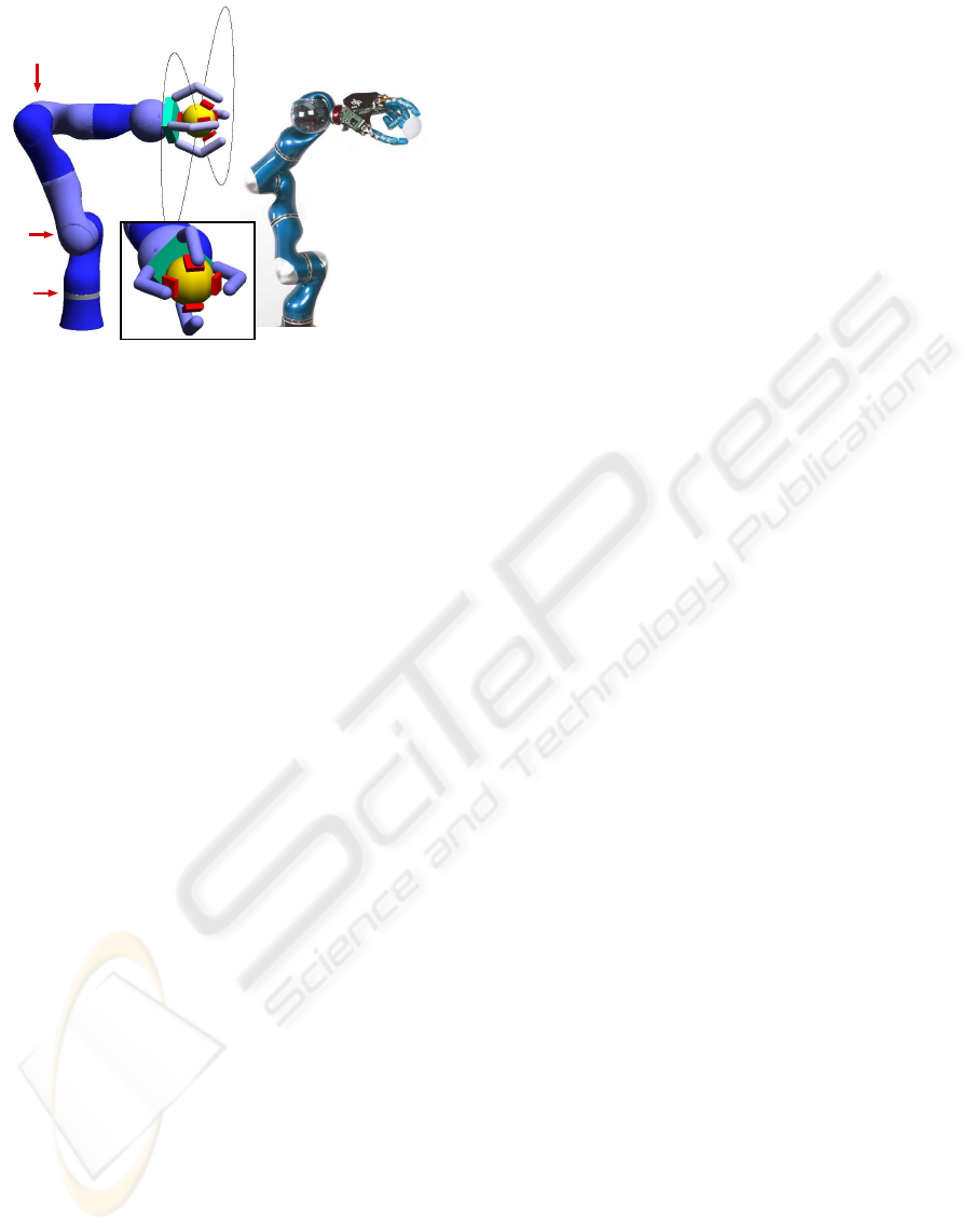
Figure 1: Simulated robot arm with gripper and force sen-
sors and its real counterpart, the DLR light-weight arm III.
Arrows indicate the three active joints used for the exper-
iments. The curve illustrates the desired trajectory of the
ball.
torques the tactile forces exerted by the manipulated
object. The same inference as above can be carried
out given that the tactile forces are linear in the ob-
ject’s mass. We demonstrate both of these steps with
mass as the varying context. If more context variables
are changing, estimating only the mass as hidden con-
text is insufficient. Particularly, if also the mass dis-
tribution changes, both the center of mass and iner-
tia tensor vary, leading to a high-dimensional latent
variable space, in which inference may be infeasible
given a limited number of data points.
In our third strategy, we use a direct mapping from
robot state, joint accelerations, and tactile forces onto
control torques. This mapping allows accurate con-
trol even with more than one changing context vari-
able and without the need to extract these variables
explicitly.
The remainder of this article is organized as fol-
lows. Section 2 briefly introduces the learning of in-
verse models under varying context. Section 3 de-
scribes the inference of inertia parameters based only
on dynamic data. Section 4 describes the inference
of mass using tactile forces. Section 5 motivates the
direct mapping. Section 6 describes the methods for
the simulation experiments. Section 7 shows the re-
sults of these experiments; and Section 8 concludes
the article.
2 LEARNING DYNAMICS
Complex robot structure and non-rigid body dynam-
ics (e.g, due to hydraulic actuation) can make analytic
solutions to the dynamics inaccurate and cumbersome
to derive. Thus, in our approach, we learn the dy-
namics for control from movement data. Particularly,
we learn an inverse model, which maps the robot’s
state (here, joint angles θ and their velocities
˙
θ) and
its desired change (joint accelerations
¨
θ) onto the mo-
tor commands (joint torques τ) that are required to
produce this change,
τ = µ(θ,
˙
θ,
¨
θ) . (1)
Under varying context, learning (1) is insufficient.
Here, the inverse model depends on a context variable
π,
τ = µ(θ,
˙
θ,
¨
θ, π) , (2)
In Sections 3 and 4, we first infer the hidden context
variable and then plug this variable into function (2) to
compute the control torques. In Section 5, the context
variable π is replaced by sensory input that implicitly
contains the hidden context.
3 INFERRING CONTEXT FROM
DYNAMICS
During robot control, hidden inertia parameters can
be inferred by observing control torques and cor-
responding accelerations (Petkos and Vijayakumar,
2007). This inference can be carried out efficiently
because of a linear relationship in the dynamics, as
shown in the following.
3.1 Linearity in Robot Dynamics
The control torques τ of a manipulator are linear in
the inertia parameters of its links (Sciavicco and Si-
ciliano, 2000). Thus, µ can be decomposed into
τ = Φ(θ,
˙
θ,
¨
θ)π . (3)
Here, π contains the inertia parameters,
π = [m
1
, m
1
l
1x
, m
1
l
1y
, m
1
l
1z
, J
1xx
, J
1xy
, ..., m
n
,
m
n
l
nx
, m
n
l
ny
, m
n
l
nz
, J
nxx
, ..., J
nzz
], where m
i
is the
mass of link i, l
i
its center-of-mass, and J
i
its inertia
tensor. The dynamics of a robot holding different
objects only differs in the π parameters of the combi-
nation of object and end-effector link (the robot’s link
in contact with the object). To obtain Φ, we need to
know for a set of contexts c the inertia parameters π
c
and the corresponding torques τ
c
. Given a sufficient
number of τ
c
and π
c
values, we can compute Φ
using ordinary least squares. After computing Φ, the
robot’s dynamics can be adjusted to different contexts
by multiplying Φ with the inertia parameters π. The
SENSOR-ASSISTED ADAPTIVE MOTOR CONTROL UNDER CONTINUOUSLY VARYING CONTEXT
263

following two sections show how to estimate π once
Φ has been found.
3.2 Inference of Inertia Parameters
Given the linear equation (3) and the knowledge of
Φ, the inertia parameters π can be inferred. Assum-
ing Gaussian noise in the torques τ, the probability
density p(τ|θ,
˙
θ,
¨
θ, π) equals
p(τ|θ,
˙
θ,
¨
θ, π) =
N (Φπ, Σ) , (4)
where N is a Gaussian function with mean Φπ and
covariance Σ. Given p(τ|θ,
˙
θ,
¨
θ, π), the most probable
inertia parameters π can be inferred using Bayes’ rule,
e.g., by assuming a constant prior probability p(π):
p(π|τ, θ,
˙
θ,
¨
θ) ∝ p(τ|θ,
˙
θ,
¨
θ, π) . (5)
3.3 Temporal Correlation of Inertia
Parameters
The above inference ignores the temporal correlation
of the inertia parameters. Usually, however, context
changes infrequently or only slightly. Thus, we may
describe the context π at time step t + 1 as a small
random variation of the context at the previous time
step:
π
t+1
= π
t
+ ε
t+1
, (6)
where ε is a Gaussian-distributed random variable
with constant covariance Ω and zero mean. Thus, the
transition probability p(π
t+1
|π
t
) is given as
p(π
t+1
|π
t
) =
N (π
t
, Ω) . (7)
Given the two conditional probabilities (4) and (7),
the hidden variable π can be described with a Markov
process (Fig. 2), and the current estimate π
t
can be
updated using a Kalman filter (Kalman, 1960). Writ-
ten with probability distributions, the filter update is
p(π
t+1
|τ
t+1
, x
t+1
) = η p(τ
t+1
|x
t+1
, π
t+1
)
·
p(π
t+1
|π
t
)p(π
t
|τ
t
, x
t
)dπ
t
, (8)
where η is a normalization constant, and x stands for
{θ,
˙
θ,
¨
θ} to keep the equation compact. A variable
with superscript t stands for all observations (of that
variable) up to time step t.
3.4 Special Case: Inference of Mass
We will demonstrate the above inference in the case of
object mass m as the hidden context. This restriction
...
τ
t
π
t
x
t+1
π
t+1
τ
t+1
x
t
...
Figure 2: Hidden Markov model for dependence of torques
τ on context π. Here, the state and state transitions are com-
bined to a vector x = {θ,
˙
θ,
¨
θ}.
essentially assumes that the shape and center of mass
of the manipulated object are invariant. If m is the
only variable context
1
, the dynamic equation is linear
in m,
τ = g(θ,
˙
θ,
¨
θ) +mh(θ,
˙
θ,
¨
θ) . (9)
In our experiments, we first learn two mappings
τ
1
(θ,
˙
θ,
¨
θ) and τ
2
(θ,
˙
θ,
¨
θ) for two given contexts m
1
and m
2
. Given these mappings, g and h can be com-
puted.
To estimate m, we plug (4) and (7) into the fil-
ter equation (8) and use (9) instead of (3). Further-
more, we assume that the probability distribution of
the mass at time t is a Gaussian with mean m
t
and
variance Q
t
. The resulting update equations for m
t
and Q
t
are
m
t+1
=
h
T
Σ
−1
(τ−g) +
m
t
Q
t
+Ω
1
Q
t
+Ω
+ h
T
Σ
−1
h
, (10)
Q
t+1
=
1
Q
t
+ Ω
+ h
T
Σ
−1
h
−1
. (11)
Section 7 demonstrates the result for this inference
of m during motor control. For feed-forward control,
we plug the inferred m into (9) to compute the joint
torques τ.
4 INFERRING CONTEXT FROM
TACTILE SENSORS
For inferring context, tactile forces measured at the
interface between hand and object may serve as a sub-
stitute for the control torques. We demonstrate this in-
ference for the special case of object mass as context.
1
This assumption is not exactly true in our case. A
changing object mass also changes the center of mass and
inertia tensor of the combination end-effector link plus ob-
ject. Here, to keep the demonstration simple, we make a
linear approximation and ignore terms of higher order in m
– the maximum value of m was about one third of the mass
of the end-effector link.
ICINCO 2007 - International Conference on Informatics in Control, Automation and Robotics
264
The sensory values s
i
(the tactile forces) are linear
in the mass m held in the robot’s hand, as shown in the
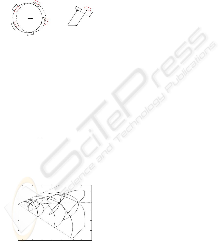
following. In the reference frame of the hand, the ac-
celeration a of an object leads to a small displacement
dx (Fig. 3).
Object
dx
dx
u
h
Sensor
Figure 3: A force on the object held in the robot’s hand
leads to a displacement dx. This displacement shifts each
sensor at position u (relative to the object’s center) by h.
This displacement pushes each sensor by the
amount h
i
depending on the sensor’s position u
i
. Let
e
i
be a vector of unit length pointing in the direction
of u
i
, then h
i
= e
T
i
dx. Our sensors act like Hookean
springs; thus, the resulting force equals f
i
= κh
i
e
i
,
with κ being the spring constant. Since the object is
held such that it cannot escape the grip, the sum of
sensory forces f
i
must equal the inertial force ma,
ma =
n
∑
i=1
f
i
= κ
∑
i
(e
T
i
dx) e
i
. (12)
This linear equation allows the computation of dx,
dx =
m
κ
(E
T
E)
−1
a , (13)
where E is a matrix with row vectors e
i
. Thus, each
f
i
is proportional to m. The total force measured at a
sensor equals f
i
plus a constant grip force (whose sum
over all sensors equals zero). Therefore, the sensory
values s can be written as
0.007
0.008
0.009
0.01
0.011
0.012
0.011 0.012 0.013 0.014 0.015 0.016 0.017 0.018
sensor 2
sensor 1
Figure 4: Two-dimensional projection of sensor values dur-
ing figure-8 movements with four different masses. From
left to right, the mass increases as 0.005, 0.01, 0.02, and
0.03.
s = s
0
+ mϕ(θ,
˙
θ,
¨
θ) , (14)
where ϕ is a function depending on the state and ac-
celeration of the robot arm. This linearity is illus-
trated in Fig. 4 using data from our simulated sensors.
Based on (14), the same inference as in Section 3 is
possible using (10) and (11), and the estimated m can
be used for control by using (9).
5 DIRECT MAPPING
The above inference of mass fails if we have addi-
tional hidden context variables, e.g., if the robot hand
holds a dumb-bell, which can swing. In this general
case, we could still use the inference based on dy-
namics. However, since for the combination of end-
effector and object, both the inertia tensor and the cen-
ter of mass vary, we need to estimate 10 hidden con-
text variables (Sciavicco and Siciliano, 2000). Given
the limited amount of training data that we use in our
experiments, we expect that inference fails in such a
high-dimensional latent space.
As alternative, we suggest using the sensory val-
ues as additional input for learning feed-forward
torques. Thus, the robot’s state and desired acceler-
ation are augmented by the sensory values, and this
augmented input is directly mapped on the control
torques. This step avoids inferring unknown hidden
variables, which are not our primary interest; our
main goal is computing control torques under vary-
ing context.
The sum of forces measured at the tactile sensors
equals the force that the manipulated object exerts
on the robotic hand. This force combined with the
robot’s state and desired acceleration is sufficient in-
formation for predicting the control torques. Thus,
tactile forces contain the relevant effects of an un-
known varying context. This context may be, e.g.,
a change in mass, a change in mass distribution, or
a human exerting a force on the object held by the
robot.
Depending on the number of sensors, the sensory
input may be high-dimensional. However, since the
sensors encode only a force vector, the intrinsic di-
mensionality is only three. For learning the mapping
τ(θ,
˙
θ,
¨
θ, s), regression techniques exist, like locally-
weighted projection regression (Vijayakumar et al.,
2005), that can exploit this reduced intrinsic dimen-
sionality efficiently. In the following, we demonstrate
the validity of our arguments in a robot-arm simula-
tion.
SENSOR-ASSISTED ADAPTIVE MOTOR CONTROL UNDER CONTINUOUSLY VARYING CONTEXT
265
6 ROBOT SIMULATION
This section describes the methods: the simulated
robot, the simulated tactile sensors, the control tasks,
the control architecture, and the learning of the feed-
forward controller.
6.1 Simulated Robot Arm
Our simulated robot arm replicates the real Light-
Weight Robot III designed by the German Aerospace
Center, DLR (Fig. 1). The DLR arm has seven
degrees-of-freedom; however, only three of them
were controlled in the present study; the remain-
ing joints were stiff. As end-effector, we attached a
simple gripper with four stiff fingers; its only pur-
pose was to hold a spherical object tightly with the
help of five simulated force sensors. The physics
was computed with the Open Dynamics Engine
(
http://www.ode.org
).
6.2 Simulated Force Sensors
Our force sensors are small boxes attached to damped
springs (Fig. 1). In the simulation, damped springs
were realized using slider joints, whose positions
were adjusted by a proportional-derivative controller.
The resting position of each spring was set such that
it was always under pressure. As sensor reading s,
we used the current position of a box (relative to the
resting position).
6.3 Control Tasks
We used two tasks: moving a ball around an eight fig-
ure and swinging a dumb-bell. In the first, one context
variable was hidden, the mass of the ball. The maxi-
mum mass (m = 0.03) of a ball was about one seventh
of the total mass of the robot arm. In the second task,
two variables were hidden: the dumb-bell mass and
its orientation. The two ball masses of the dumb-bell
were equal.
In all tasks, the desired trajectory of the end-
effector was pre-defined (Figs. 1 and 5) and its in-
verse in joint angles pre-computed. The eight was
traversed only once lasting 5000 time steps, and for
the dumb-bell, the end-effector swung for two peri-
ods together lasting 5000 time steps and followed by
1000 time steps during which the end-effector had to
stay in place (here, the control torques need to com-
pensate for the swinging dumb-bell). In both tasks,
a movement started and ended with zero velocity and
acceleration. The velocity profile was sinusoidal with
one peak.
For each task, three trajectories were pre-
computed: eight-figures of three different sizes (Fig.
1 shows the big eight; small and medium eight are 0.9
and 0.95 of the big-eight’s size, see Fig. 11) and three
lines of different heights (Fig. 13). For training, data
points were used from the two extremal trajectories,
excluding the middle trajectory. For testing, all three
trajectories were used.
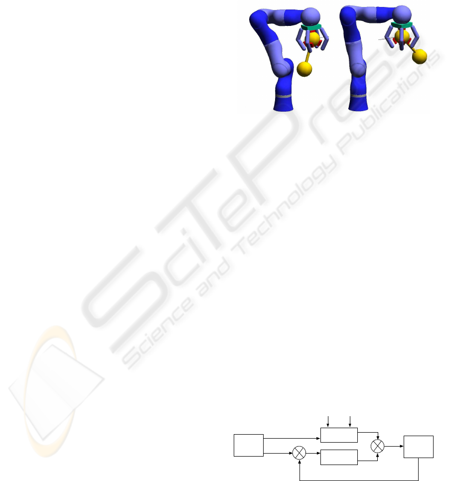
Figure 5: Robot swinging a dumb-bell. The black line
shows the desired trajectory.
6.4 Control Architecture
We used an adaptive controller and separated train-
ing and test phases. To generate training patterns, a
proportional-integral-derivative (PID) controller pro-
vided the joint torques. The proportional gain was
chosen to be sufficiently high such that the end-
effector was able to follow the desired trajectories.
The integral component was initialized to a value that
holds the arm against gravity (apart from that, its ef-
fect was negligible).
For testing, a composite controller provided the
joint torques (Fig. 6). The trained feed-forward con-
troller was put in parallel with a low-gain error feed-
back (its PD-gain was 1% of the gain used for training
in the ball case and 4% in the dumb-bell case). For
those feed-forward mappings that require an estimate
of the object’s mass, this estimate was computed us-
ing a Kalman filter as described above (the transition
Motion
plan
Controller
Plant
+
_
+
+
θ
d
.
θ
d
..
θ
d
θ
d
.
θ
d
.
θ
τ
ff
fb
τ
τ
Sensorm
or
θ
PD
Figure 6: Composite control for the robot arm. A feed-
forward controller is put in parallel with error feed-back
(low PD gain).
ICINCO 2007 - International Conference on Informatics in Control, Automation and Robotics
266
noise Ω of m was set to 10
−9
for both dynamics and
sensor case).
6.5 Controller Learning
The feed-forward controller was trained on data col-
lected during pure PID-control. For each mass con-
text, 10000 data points were collected in the ball case
and 12000 data points in the dumb-bell case. Half
of these points (every second) were used for training
and the other half for testing the regression perfor-
mance. Three types of mappings were learned. The
first maps the state and acceleration values (θ,
˙
θ,
¨
θ)
onto joint torques. The second maps the same input
onto the five sensory values, and the third maps the
sensor augmented input (θ,
˙
θ,
¨
θ, s) onto joint torques.
The first two of these mappings were trained on two
different labeled masses (m
1
= 0.005 and m
2
= 0.03
for ball or m
2
= 0.06 for dumb-bell). The last map-
ping used the data from 12 different mass contexts (m
increased from 0.005 to 0.06 in steps of 0.005); here,
the contexts were unlabeled.
Our learning task requires a non-linear regres-
sion technique that provides error boundaries for each
output value (required for the Kalman-filtering step).
Among the possible techniques, we chose locally-
weighted projection regression (LWPR)
2
(Vijayaku-
mar et al., 2005) because it is fast – LWPR is O(N),
where N is the number of data points; in contrast,
the popular Gaussian process regression is O(N
3
) if
making no approximation (Rasmussen and Williams,
2006).
7 RESULTS
The results of the robot-simulation experiments are
separated into ball task – inference and control under
varying mass – and dumb-bell task – inference and
control under multiple varying context variables.
7.1 Inference and Control Under
Varying Mass
For only one context variable, namely the mass of the
manipulated object, both inference strategies (Sec-
2
LWPR uses locally-weighted linear-regression. Data
points are weighted according to Gaussian receptive fields.
Our setup of the LWPR algorithm was as follows. For each
output dimension, a separate LWPR regressor was com-
puted. The widths of the Gaussian receptive fields were
hand-tuned for each input dimension, and these widths were
kept constant during the function approximation. Other
learning parameters were kept at default values.
tions 3 and 4) allowed to infer the unknown mass ac-
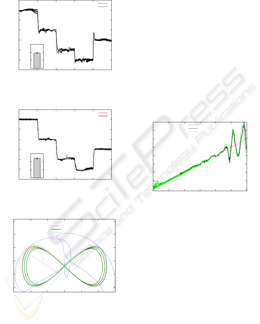
curately (Figs. 7 to 10).
-0.005
0
0.005
0.01
0.015
0.02
0.025
0.03
0.035
0 1000 2000 3000 4000 5000
mass
time step
true mass
dynamic estimate
0
0.01
0.02
0.03
nMSE
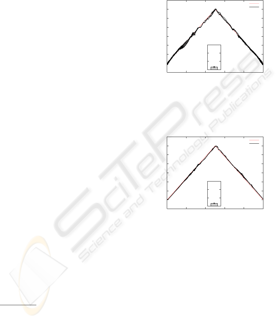
Figure 7: Inferring mass purely from dynamics. The in-
ference results are shown for all three trajectories. The in-
set shows the normalized mean square error (nMSE) of the
mass estimate. The error bars on the nMSE are min and
max values averaged over an entire trajectory.
-0.005
0
0.005
0.01
0.015
0.02
0.025
0.03
0.035
0 1000 2000 3000 4000 5000
mass
time step
true mass
sensor estimate
0
0.01
0.02
0.03
nMSE
Figure 8: Inferring mass using tactile sensors. For details
see Fig. 7.
Both types of mappings from state and acceler-
ation either onto torques or onto sensors could be
learned with low regression errors, which were of
the same order (torques with m = 0.005: normalized
mean square error (nMSE) = 2.9 ∗ 10
−4
, m = 0.03:
nMSE = 2.7∗ 10
−4
; sensors with m = 0.005: nMSE =
1.3∗ 10
−4
, m = 0.03: nMSE = 2.2∗ 10
−4
). The error
of the inferred mass was about the same for dynamics
and sensor pathway. However, the variation between
trials was lower in the sensor case.
Given the inferred mass via the torque and sensory
pathways (Sections 3 and 4), our controller could pro-
vide accurate torques (Fig. 11). The results from both
pathways overlap with the desired trajectory. As illus-
trated in the figure, a PID controller with a PD-gain
as low as the gain of the error feed-back for the com-
SENSOR-ASSISTED ADAPTIVE MOTOR CONTROL UNDER CONTINUOUSLY VARYING CONTEXT
267
0
0.005
0.01
0.015
0.02
0.025
0.03
0.035
0 1000 2000 3000 4000 5000
mass
time step
true mass
dynamic estimate
0
0.01
0.02
0.03
nMSE
Figure 9: Inferring mass purely from dynamics. For details
see Fig. 7.
0
0.005
0.01
0.015
0.02
0.025
0.03
0.035
0 1000 2000 3000 4000 5000
mass
time step
true mass
sensor estimate
0
0.01
0.02
0.03
nMSE
Figure 10: Inferring mass using tactile sensors. For details
see Fig. 7.
0.4
0.6
0.8
1
1.2
1.4
-0.6 -0.4 -0.2 0 0.2 0.4 0.6
z-coordinate
y-coordinate
target
low-gain PID
sensor estimate
dynamic estimate
wrong mass
Figure 11: Following-the-eight task. The figure com-
pares low-gain PID control (on large eight only) with the
composite-controller that uses either the predicted mass es-
timate (from dynamics or sensors) or a wrong estimate
(m = 0.03, on large eight only). The true mass decreased
continuously from 0.03 to 0. The results for composite con-
trol based on the predicted mass overlap with the target for
all three test curves.
posite controller was insufficient for keeping the ball
on the eight figure. The figure furthermore illustrates
that without a correct mass estimate, tracking was im-
paired. Thus, correctly estimating the mass matters
for this task.
7.2 Inference and Control Under
Multiple Varying Context
The inference of mass based on a single hidden vari-
able failed if more variables varied (Fig. 12). We
demonstrate this failure with the swinging dumb-bell,
whose mass increased continuously during the trial.
In the last part of the trial, when the dumb-bell was
heavy and swung, the mass inference was worst. The
wrong mass estimate further impaired the control of
the robot arm (see Fig. 13).
0
0.01
0.02
0.03
0.04
0.05
0.06
0.07
0.08
0 1000 2000 3000 4000 5000 6000
mass
time step
true mass
sensor estimate
dynamic estimate
Figure 12: Inference of mass in the dumb-bell task.
During the last part of the movement, tracking was
better with the direct mapping from (θ,
˙
θ,
¨
θ, s) onto
torques. For this mapping, the results still show some
deviation from the target. However, we expect this
error to reduce with more training data.
8 CONCLUSIONS
We presented three strategies for adaptive motor con-
trol under continuously varying context. First, hidden
inertia parameters of a manipulated object can be in-
ferred from the dynamics and in turn used to predict
control torques. Second, the hidden mass of an object
can be inferred from the tactile forces exerted by the
object. Third, correct control torques can be predicted
by augmenting the input (θ,
˙
θ,
¨
θ) with tactile forces
and by directly mapping this input onto the torques.
We demonstrated the first two strategies with ob-
ject mass as the varying context. For more context
ICINCO 2007 - International Conference on Informatics in Control, Automation and Robotics
268
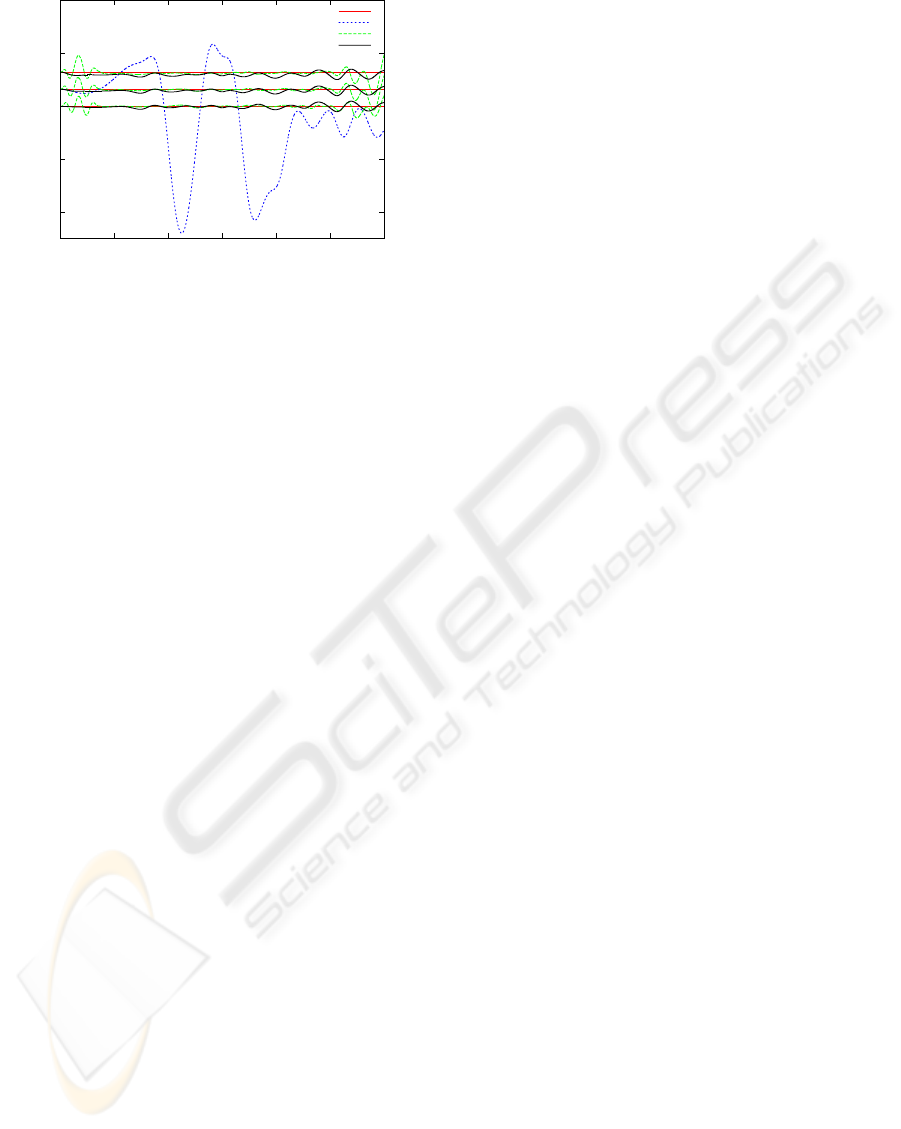
0.52
0.53
0.54
0.55
0.56
0 1000 2000 3000 4000 5000 6000
z-coordinate
time step
target
low-gain PID
dynamic estimate
direct mapping
Figure 13: Swinging-the-dumb-bell task. The figure com-
pares low-gain PID control (shown only on the middle tra-
jectory) with the composite-controller that uses either the
predicted mass estimate from dynamics or a direct mapping
from (θ,
˙
θ,
¨
θ, s) onto torques. For the estimate from sen-
sors, the results were similar to the dynamics case and are
omitted in the graph to improve legibility. The true mass
increased continuously from 0 to 0.06.
variables, inferring the mass failed, and thus, the con-
trol torques were inaccurate. In principle, all iner-
tia parameters could be inferred from the dynamics,
but this inference requires modeling a 10-dimensional
latent-variable space, which is unfeasible without ex-
tensive training data.
On the other hand, the direct mapping onto
torques with sensors as additional input could predict
accurate control torques under two varying context
variables and in principle could cope with arbitrary
changes of the manipulated object (including exter-
nal forces). Further advantages of this strategy are its
simplicity (it only requires function approximation),
and for training, no labeled contexts are required.
In future work, we try to replicate these findings
on a real robot arm with real tactile sensors. Real sen-
sors might be more noisy compared to our simulated
sensors; particularly, the interface between sensor and
object is less well controlled.
ACKNOWLEDGEMENTS
The authors are grateful to the German Aerospace Center
(DLR) for providing the data of the Light-Weight Robot III
and to Marc Toussaint and Djordje Mitrovic for their con-
tribution to the robot-arm simulator. This work was funded
under the SENSOPAC project. SENSOPAC is supported
by the European Commission through the Sixth Framework
Program for Research and Development up to 6 500 000
EUR (out of a total budget of 8 195 953.50 EUR); the SEN-
SOPAC project addresses the “Information Society Tech-
nologies” thematic priority. G. P. was funded by the Greek
State Scholarships Foundation.
REFERENCES
Haruno, M., Wolpert, D. M., and Kawato, M. (2001).
Mosaic model for sensorimotor learning and control.
Neural Computation, 13:2201–2220.
Kalman, R. E. (1960). A new approach to linear filtering
and prediction problems. Transactions of the ASME -
Journal of Basic Engineering, 82:35–45.
Narendra, K. S. and Balakrishnan, J. (1997). Adaptive con-
trol using multiple models. IEEE Transactions on Au-
tomatic Control, 42(2):171–187.
Narendra, K. S. and Xiang, C. (2000). Adaptive con-
trol of discrete-time systems using multiple mod-
els. IEEE Transactions on Automatic Control,
45(9):1669–1686.
Petkos, G., Toussaint, M., and Vijayakumar, S. (2006).
Learning multiple models of non-linear dynamics for
control under varying contexts. In Proceedings of
the International Conference on Artificial Neural Net-
works. Springer.
Petkos, G. and Vijayakumar, S. (2007). Context estimation
and learning control through latent variable extraction:
From discrete to continuous contexts. In Proceedings
of the International Conference on Robotics and Au-
tomation. IEEE.
Rasmussen, C. E. and Williams, C. K. I. (2006). Gaussian
Processes for Machine Learning. MIT Press.
Sciavicco, L. and Siciliano, B. (2000). Modelling and Con-
trol of Robot Manipulators. Springer.
Vijayakumar, S., D’Souza, A., and Schaal, S. (2005). In-
cremental online learning in high dimensions. Neural
Computation, 17:2602–2634.
Wolpert, D. M. and Kawato, M. (1998). Multiple paired
forward and inverse models for motor control. Neural
Networks, 11:1317–1329.
SENSOR-ASSISTED ADAPTIVE MOTOR CONTROL UNDER CONTINUOUSLY VARYING CONTEXT
269
