
MODELING AND OPTIMAL TRAJECTORY PLANNING OF A
BIPED ROBOT USING NEWTON-EULER FORMULATION
David Tlalolini, Yannick Aoustin and Christine Chevallereau
Institut de Recherche en Communications et Cybern
´
etique de Nantes
CNRS, Ecole Centrale de Nantes, Universit de Nantes, 1 rue la No, 44321 Nantes, France
Keywords:
3D biped, cyclic walking gait, parametric optimization, constraints.
Abstract:
The development of an algorithm to achieve optimal cyclic gaits in space for a thirteen-link biped and twelve
actuated joints is proposed. The cyclic walking gait is composed of successive single support phases and
impulsive impacts with full contact between the sole of the feet and the ground. The evolution of the joints are
chosen as spline functions. The parameters to define the spline functions are determined using an optimization
under constraints on the dynamic balance, on the ground reactions, on the validity of impact, on the torques
and on the joints velocities. The criterion considered is represented by the integral of the torque norm. The
algorithm is tested for a biped robot whose numerical walking results are presented.
1 INTRODUCTION
The design of walking gaits for legged robots and par-
ticularly the bipeds has attracted the interest of many
researchers for several decades. Due to the unilateral
constraints of the biped with the ground and the great
number of degrees of freedom, this problem is not
trivial. Intuitive methods can be used to obtain walk-
ing gaits as in (Grishin et al., 1994). Using experi-
mental data and physical considerations, the authors
defined polynomial functions in time for a prototype
planar biped. This method is efficient. However to
build a prototype and to choose the appropriate actu-
ators or to improve the autonomy of a biped, an op-
timization algorithm can lead to very interesting re-
sults. In (Rostami and Besonnet, 1998) the Pontrya-
gin’s principle is used to design impactless nominal
trajectories for a planar biped with feet. However the
calculations are complex and difficult to extend to the
3D case. As a consequence a parametric optimisation
is a useful tool to find optimal motion.
The choice of optimisation parameters is not
unique. The torques, the Cartesian coordinates or
joint coordinates can be used. Discrete values for the
torques defined at sampling time are used as optimiza-
tion parameters in (Roussel et al., 2003). However
it is necessary, when the torque is an optimised vari-
able, to solve the inverse dynamic problem to find the
joint accelerations and integrations are used to obtain
the evolution of the reference trajectory in velocity
and in position. Thus this approach require many cal-
culation : the direct dynamic model is complex and
many evaluations of this model is used in the inte-
gration process. In (Beletskii and Chudinov, 1977),
(Bessonnet et al., 2002), (Channon et al., 1992), (Zon-
frilli et al., 2002), (Chevallereau. and Aoustin, 2001)
or (Miossec and Aoustin, 2006) to overcome this diffi-
culty, the parametric optimization defines directly the
reference trajectories of Cartesian coordinates or joint
coordinates for 2D bipeds with feet or without feet.
An extension of this strategy is given in this paper for
a 3D biped with with twelve motorized joints. The
dynamic model is more complex than for a 2D biped,
so its computation cost is important in the optimisa-
tion process and the use of Newton-Euler method to
calculate the torque is more appropriate than the La-
grange method usually used. Since the inverse dy-
namic model is used only to evaluate the torque for
the constraints and criterion calculation, the number
of evaluation of the torque can be limited. The de-
sired motion is based on the solution of an optimal
problem whose constraints depend on the nonlinear
multibody system dynamics of the 12 DoF biped and
physical contact constraints with the environment.
76
Tlalolini D., Aoustin Y. and Chevallereau C. (2007).
MODELING AND OPTIMAL TRAJECTORY PLANNING OF A BIPED ROBOT USING NEWTON-EULER FORMULATION.
In Proceedings of the Fourth International Conference on Informatics in Control, Automation and Robotics, pages 76-83
DOI: 10.5220/0001628200760083
Copyright
c
SciTePress

A half step of the cyclic walking gait is com-
posed uniquely of a single support and an instanta-
neous double support that is modelled by passive im-
pulsive equations. This walking gait is simpler that
the human gait, but with this simple model the cou-
pling effect between the motion in frontal plan and
sagittal plane can be studied. A finite time double
support phase in not considered in this work currently
because for rigid modelling of robot, a double support
phase can usually be obtained only when the velocity
of the swing leg tip before impact is null. This con-
straint has two effects. In the control process it will
be difficult to touch the ground with a null velocity,
as a consequence the real motion of the robot will be
far from the ideal cycle. Furthermore, large torques
are required to slow down the swing leg before the
impact and to accelerate the swing leg at the begin-
ning of the single support. The energy cost of such
a motion is higher than a motion with impact in the
case of a planar robot without feet (Chevallereau. and
Aoustin, 2001), (Miossec and Aoustin, 2006).
Therefore a dynamic model is calculated for the
single phase. An impulsive model for the impact on
the ground with complete surface of the foot sole of
the swing leg is deduced from the dynamic model
for the biped in double support phase. It takes into
account the wrench reaction from the ground. This
model is founded on the Newton Euler algorithm,
considering that the reference frame is connected to a
stance foot. The evolution of joint variables are cho-
sen as a spline function of time instead of usual poly-
nomial functions to prevent oscillatory phenomenon
during the optimization process (see (Chevallereau.
and Aoustin, 2001), (Saidouni and Bessonnet, 2003)
or (L. Hu and Sun, 2006)). The coefficients of the
spline functions are calculated as function of initial,
intermediate and final configurations and initial and
final velocities of the robot which are optimization
variables. Taking into account the impact and the fact
that the desired walking gait is cyclic, the number of
optimization variables is reduced. The criterion con-
sidered is the integral of the torque norm. During the
optimization process, the constraints on the dynamic
balance, on the ground reactions, on the validity of
impact, on the limits of the torques, on the joints ve-
locities and on the motion velocity of the biped robot
are taken into account. The paper is organized as fol-
lows. The 3D biped and its dynamic model are pre-
sented in Section II. The cyclic walking gait and the
constraints are defined in Section III. The optimiza-
tion parameters, optimization process and the crite-
rion are discussed in Section IV. Simulation results
are presented in Section V. Section VI contains our
conclusion and perspectives.
2 MODELS OF THE STUDIED
BIPED ROBOT
2.1 Biped Model
We considered an anthropomorphic biped robot with
thirteen rigid links connected by twelve motorized
joints to form a tree structure. It is composed of a
torso, which is not directly actuated, and two identi-
cal open chains called legs that are connected at the
hips. Each leg is composed of two massive links con-
nected by a joint called knee. The link at the extremity
of each leg is called foot which is connected at the leg
by a joint called ankle. Each revolute joint is assumed
to be independently actuated and ideal (frictionless).
The ankles of the biped robot consist of the pitch and
the roll axes, the knees consist of the pitch axis and
the hips consist of the roll, pitch and yaw axes to con-
stitute a biped walking system of two 2-DoF ankles,
two 1-DoF knees and two 3-DoF hips as shown in
figure 1. The action to walk associates single support
phases separated by impacts with full contact between
the sole of the feet and the ground, so that a model in
single support, a model in double support and an im-
pact model are derived.
2.2 Geometric Description of the Biped
To define the geometric structure of the biped walk-
ing system we assume that the link 0 (stance foot)
is the base of the biped robot while link 12 (swing
foot) is the terminal link. Therefore we have a sim-
ple open loop robot which geometric structure can be
described using the notation of Khalil and Kleinfinger
(Khalil and Dombre, 2002). The definition of the link
frames is given in figure 1 and the corresponding ge-
ometric parameters are given in Table I. The frame R
0
coordinates, which is fixed to the tip of the right foot
(determined by the width l
p
and the length L
p
), is de-
fined such that the axis z
0
is along the axis of frontal
joint ankle. The frame R
13
is fixed to the tip of the left
foot in the same way that R
0
.
2.3 Dynamic Model in Single Support
Phase
During the single support phase the stance foot is as-
sumed to remain in flat contact on the ground, i.e.,
no sliding motion, no take-off, no rotation. Therefore
the dynamics of the biped is equivalent to an 12 DoF
manipulator robot. Let q ∈ R
12
be the generalized co-
ordinates, where q
1
,...,q
12
denote the relative angles
of the joints, ˙q ∈ R
12
and ¨q ∈ R
12
are the velocity
MODELING AND OPTIMAL TRAJECTORY PLANNING OF A BIPED ROBOT USING NEWTON-EULER
FORMULATION
77
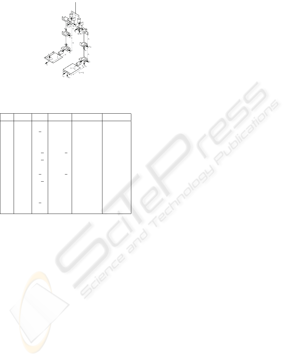
Figure 1: The multi-body model and link frames of the
biped robot.
Table 1: Geometric parameters of the biped.
j a( j) α
j
θ
j
r
j
d
j
1 0 0 q
1
l
1
d
1
2 1
π
2
q
2
0 0
3 2 0 q
3
0 d
3
4 3 0 q
4
l
4
d
4
5 4 −
π
2
q
5
−
π
2
0 0
6 5 −
π
2
q
6
0 0
7 6 0 q
7
0 d
7
8 7
π
2
q
8
−
π
2
0 0
9 8 −
π
2
q
9
0 0
10 9 0 q
10
l
10
= l
4
d
10
= d
4
11 10 0 q
11
0 d
11
= d
3
12 11
π
2
q
12
0 0
13 12 0 q
13
l
13
= −l
1
d
13
= d
1
and acceleration vectors respectively. The dynamic
model is computed using the Newton-Euler method
(see (Khalil and Dombre, 2002)) represented by the
following relation
Γ = f(q, ˙q, ¨q,F
t
) (1)
where Γ ∈ R
12
is the joint torques vector and F
t
is
the external wrench (forces and torques), exerted by
the swing foot on the ground. In single support phase
F
t
= 0 and in double support phase F
t
6= 0.
In order to denote the dynamic model under the
Lagrange form
Γ = D
s
(q) ¨q+ H
s
(2)
with
H
s
= (C
s
(q, ˙q) + G
s
(q)) (3)
the equation (1) is used. In such calculation the ma-
trix D
s
and the vector H
s
are needed. C
s
∈ R
12
repre-
sents the Coriolis and centrifugal forces and G
s
∈ R
12
is the vector of gravity.
The matrix D
s
is calculated by the algorithm
of Newton-Euler, by noting from the relation (1),
(M.W.Walker and D.E.Orin, 1982), that the i
th
col-
umn is equal to Γ if
˙q = 0,g = 0, ¨q = e
i
,F
t
= 0
e
i
∈ R
12×1
is the unit vector, whose elements are zero
except the i
th
element which is equal to 1.
The calculation of the vector H
s
is obtained in the
same way that D
s
considering that H
s
= Γ if ¨q = 0.
Therefore, the dynamic model under the Lagrange
form is denoted by the following matrix equations
Γ = D
s
(q) ¨q+ H
s
(q, ˙q)
where D
s
∈ R
12×12
is the symmetric definite positive
inertia matrix.
To take easily into account the effect of the reac-
tion force on the stance foot, it is interesting to add 6
coordinates to describe the situation of the stance foot.
Newton variables are used for this link, thus its veloc-
ity is described by the linear velocity of frame R
0
: V
0
and angular velocity ω
0
. Since the stance foot is as-
sumed to remain in flat contact, the resultant ground
reaction force/moment F
R
and M
R
are computed by
using the Newton-Euler algorithm. ω
0
= 0,
˙
ω
0
= 0
and
˙
V
0
= −g are the initial conditions of the Newton-
Euler algorithm to take into account the effect of grav-
ity. So, the equation (2) becomes
D(X)
˙
V +C(V,q) + G(X) = D
Γ
Γ+ D
R
R
F
R
(4)
where X = [X
0
,α
0
,q]
T
∈ R
18
, X
0
and α
0
is the posi-
tion and the orientation variables of frame R
0
, V =
[
0
V
0
,
0
ω
0
, ˙q]
T
∈ R
18
and
˙
V = [
0
˙
V
0
,
0
˙
ω
0
, ¨q]
T
∈ R
18
.
D ∈ R
18×18
is the symmetric definite positive iner-
tia matrix, C ∈ R
18
represents the Coriolis and cen-
trifugal forces, G ∈ R
18
is the vector of gravity.
R
F
R
= [F
R
,M
R
]
T
∈ R
6
is the ground reaction forces
on the stance foot, calculated by the Newton-Euler al-
gorithm, D
Γ
= [0
6×12
| I
12×12
]
T
∈ R
18×12
and D
R
=
[I
6×6
| 0
12×6
]
T
∈ R
6×18
are constant matrices com-
posed of 1 and 0.
In the optimization process, the torques and force
are calculated with the Newton-Euler algorithm and
not with the equation (4). The Newton-Euler is much
more efficient from the computation point of view,
(Khalil and Dombre, 2002).
2.4 Dynamic Model in Double Support
Phase
In double support phase, only the forces and moments
of interaction of the left foot with the ground have to
be added. Then, the model (4) becomes
D(X)
˙
V +C(V,q) + G(X) + D
f
R
f
= D
Γ
Γ+ D
R
R
F
R
(5)
ICINCO 2007 - International Conference on Informatics in Control, Automation and Robotics
78

where R
f
∈ R
6
represents the vector of forces F
12
and
moments M
12
exerted by the left foot on the ground.
This wrench is naturally expressed in frame R
12
:
12
F
12
,
12
M
12
. The virtual work δW
12
of this wrench is :
δW
12
=
12
F
T12
12
d
12
+
12
M
12
12
δ
12
(6)
where
12
d
12
represents an infinitesimal virtual dis-
placement of the link 12 and
12
δ
12
represents an in-
finitesimal virtual angular displacement. The relation
between these virtual displacements,
12
d
12
and
12
δ
12
,
and the virtual joints displacement δq
12
are the same
that between the velocities
12
V
12
,
12
ω
12
and ˙q
12
.
Usually the velocities of link 12 can be expressed
as
V
12
w
12
=
V
0
+ w
0
×
0
P
12
w
12
+ J
12
˙q (7)
where
0
P
12
is the vector linking the origin of frame R
0
and the origin of frame R
12
expressed in frame R
0
, J
12
∈ R
6×12
is the Jacobian matrix of the robot, J
12
˙q rep-
resents the effect of the joint velocities on the Carte-
sian velocity of link 12. The velocities V
12
and w
12
must be expressed in frame R
12
, thus we write (7):
12
V
12
12
w
12
=
12
A
0
−
12
A
0
0
ˆ
P
12
0
3×3
12
A
0
0
V
0
0
w
0
+
12
J
12
˙q
(8)
where
12
A
0
∈ R
3×3
is the rotation matrix, which de-
fines the orientation of frame R
0
with respect to frame
R
12
. Term
0
ˆ
P
12
is the skew-symmetric matrix of the
vector product associated with vector
0
P
12
.
0
ˆ
P
12
=
0 −P
z
P
y
P
z
0 −P
x
−P
y
P
x
0
Defining matrix D
f
∈ R
18×6
as the concatenation
of two matrices such that D
f
= [T |
12
J
12
]
T
, where
12
J
12
∈ R
6×12
is the Jacobian matrix of the robot and
T ∈ R
6×6
equals
T =
12
A
0
−
12
A
0
0
ˆ
P
12
0
3×3
12
A
0
(9)
Then, the linear and angular velocities of the swing
foot in frame R
12
is :
12
V
12
12
w
12
= D
T
f
V (10)
Then D
f
can be defined by applying the virtual prin-
ciple on the second leg. However in order to com-
pute the matrix D
f
, it is necessary, either to calculate
the matrix
12
J
12
jacobian by a traditional method, by
taking into account the equation (9), or to calculate
this matrix by the algorithm of Newton-Euler, by not-
ing from relation (5) that the i
th
column is equal to
D
Γ
Γ+ D
R
R
F
R
if
˙
V = 0,V = 0,g = 0 and R
f
= e
i
e
i
∈ R
6×1
is the unit vector, whose elements are zero
except the i
th
element which is equal to 1.
2.5 Impact Equations for Instantaneous
Double Support
When the swing foot touches the ground, an impact
exists. In reality many possibilities can appear for an
impact (partial contact with the sole on the ground,
elastic deformations of the bodies and the ground).
To simplify our study this impact is assumed to be in-
stantaneous and inelastic with complete surface of the
foot sol touching the ground. This means that the ve-
locity of the swing foot touching the ground is zero
after its impact. We assume that the ground reaction
at the instant of impact is described by a Dirac delta-
function with intensity I
R
f
. Assuming that the previ-
ous stance foot is motionless before the impact and
does not remains on the ground after the impact the
dynamic model during the impact is (see (Formal’sky,
1982) and (M. Sakaguchi and Koizumi, 1995))
D(X)∆V = −D
f
I
R
f
(11)
D
T
f
V
+
= 0 (12)
0
V
−
0
0
w
−
0
=
0
3×1
0
3×1
(13)
where ∆V = (V
+
− V
−
) is the change of velocity
caused by the impact and V
+
(respectively V
−
) de-
note the linear and angular velocity of the stance foot
and also the joint velocities of the biped after (respec-
tively before) the impact. These equations form a sys-
tem of linear equations which solution allows to know
the impulse forces and the velocity after the impact,
thus they can be applied to the biped walking system.
3 DEFINITION OF THE
WALKING CYCLE
Because biped walking is a periodical phenomenon
our objective is to design a cyclic biped gait. A com-
plete walking cycle is composed of two phases: a sin-
gle support phase and a double support phase which is
modeled through passive impact equations. The sin-
gle support phase begins with one foot which stays
on the ground while the other foot swings from the
rear to the front. We shall assume that the double sup-
port phase is instantaneous, this means that when the
swing leg touches the ground the stance leg takes off.
There are two facets to be considered for this prob-
lem. The definition of reference trajectories and the
method to determine a particular solution of it. This
section is devoted to the definition of reference tra-
jectories. The optimal process to choose the best so-
lution of parameters, allowing a symmetric half step,
MODELING AND OPTIMAL TRAJECTORY PLANNING OF A BIPED ROBOT USING NEWTON-EULER
FORMULATION
79

from the point of view of a given criterion will be de-
scribed in the next section.
3.1 Cyclic Walking Trajectory
Since the initial configuration is a double support con-
figuration, the both feet are on the ground, the twelve
joint coordinates are not independent. Because the
absolute frame is attached to the right foot we define
the situation of the left foot by (y
l f
,z
l f
,φ
l f
) and the
situation of the middle of the hips (x
h
,y
h
,z
h
,θ
h
), both
expressed in R
0
frame. (y
l f
,z
l f
) is the coordinate, in
the horizontal plane, of the left foot position, φ
l f
de-
notes the left foot yawing motion, (x
h
,y
h
,z
h
) is the
hip position and θ
h
defines the hip pitching motion.
The values of the joint variables are solution of the
inverse kinematics problem for a leg, which may also
be considered as a 6-link manipulator. The problem
is solved with a symbolic software, (SYMORO+, see
(Khalil and Dombre, 2002)).
In order to deduce the final configuration, we im-
pose a symmetric role of the two legs, therefore from
the initial configuration, the final configuration is de-
duced as:
q
f
DS
= Eq
i
DS
(14)
where E ∈ R
12×12
is an inverted diagonal matrix
which describes the legs’ exchange.
Taking into account the impulsive impact (11)-
(13), we can compute the velocity after the impact.
Therefore, the velocity after the impact, ˙q
+
, can be
calculated when the velocity before the impact, ˙q
−
, is
known. The use of the defined matrix E allows us to
calculate the initial velocity for the current half step
as:
˙q
i
= E ˙q
+
. (15)
By this way the conditions of cyclic motion are satis-
fied.
3.2 Constraints
In order to insure that the trajectory is possible, many
constraints have to be considered.
3.2.1 Magnitude Constraints on Position and
Torque
• Each actuator has physical limits such that
|
Γ
i
|
− Γ
i,max
≤ 0, for i = 1, ..., 12 (16)
where Γ
i,max
denotes the maximum value for each
actuator.
|
˙q
i
|
− ˙q
i,max
≤ 0, for i = 1, ..., 12 (17)
where ˙q
i,max
denotes the maximum velocity for
each actuator.
• The upper and lower bounds of joints for the con-
figurations during the motion are:
q
i,min
≤ q
i
≤ q
i,max
, for i = 1, ..., 12 (18)
q
i,min
and q
i,max
stands respectively for the mini-
mum and maximum joint limits.
3.2.2 Geometrical Constraints in Double
Support Phase
• The distance d(hip, foot) between the foot in
contact with the ground and the hip must remain
within a maximal value, i.e.,
d(hip, foot) ≤ l
hip
. (19)
This condition must hold for initial and final con-
figurations of the double support.
• In order to avoid the internal collision of both feet
through the lateral axis the heel and the toe of the
left foot must satisfy
y
heel
≤ −a and y
toe
≤ −a (20)
with a >
l
p
2
and and l
p
is the width of right foot.
3.2.3 Walking Constraints
• During the single support phase to avoid colli-
sions of the swing leg with the stance leg or with
the ground, constraints on the positions of the four
corners of the wing foot are defined.
• We must take into account the constraints on the
ground reaction R
F
R
= [R
F
Rx
,R
F
Ry
,R
F
Rz
]
T
for the
stance foot in single support phase as well as im-
pulsive forces I
R
f
= [I
R
fx
,I
R
fy
,I
R
fz
]
T
on the foot
touching the ground in instantaneous double sup-
port phase. The ground reaction and impulsive
forces must be inside a friction cone defined by
the friction coefficient µ. This is equivalent to
write
q
R
2
F
Ry
+ R
2
F
Rz
≤ µR
F
Rx
(21)
q
I
2
R
fy
+ I
2
R
fz
≤ µI
R
fx
(22)
The ground reaction forces and the impulsive
forces at the contact can only push the ground but
may not pull from ground, then the condition of
no take off is deduced:
R
f
x
≥ 0 (23)
I
R
fx
≥ 0. (24)
ICINCO 2007 - International Conference on Informatics in Control, Automation and Robotics
80

• In order to maintain the balance in dynamic walk-
ing, the ZMP ≡ CoP, (Zero Moment Point equiv-
alent to the Center of Pressure, see (Vukobratovic
and Stepanenko, 1972), point must be within the
support polygon, i.e., the distance from CoP to
support polygon is negative
d(CoP, SP) ≤ 0, (25)
where SP denotes the support polygon determined
by the width l
p
and the length L
p
of the feet.
4 PARAMETRIC OPTIMIZATION
4.1 The Cubic Spline
To describe the joint motion by a finite set of parame-
ters we choose to use for each joint a piecewise func-
tion of the form
q
i
= ϕ
i
(t) =
ϕ
i1
(t) i f t
0
≤ t ≤ t
1
ϕ
i2
(t) i f t
1
≤ t ≤ t
2
.
.
.
ϕ
in
(t) i f t
n−1
≤ t ≤ t
n
i = 1,...12
where ϕ
k
(t) are polynomials of third-order such that
ϕ
ik
(a
ik
,t) =
3
∑
j=0
a
ik j
(t −t
k−1
)
j
, k = 1,...,n ∀t ∈ [t
0
,t
n
]
(26)
where a
ik j
are calculated such that the position,
velocity and acceleration are always continuous in
t
0
,t
1
,...t
n
. We used n = 3, thus the motion is defined
by a specified initial configuration, a final configura-
tion in double support and two intermediate configu-
rations in single support taking into account the initial
and final velocity as boundary conditions.
4.2 Optimization Parameters
A parametric optimization problem has to be solved
to design a cyclic bipedal gait with successive single
and double support phases. This problem depends on
parameters to prescribe the two intermediate configu-
rations, q
int1
and q
int2
, and the final velocity ˙q
f
in the
single support phase. Taking into account the condi-
tions (14) and (15) the minimal number of parameters
necessary to define the joint motion are:
1. Twenty-four parameters are needed to define the
two intermediate configurations in single support
phase, twelve parameters for the first intermediate
configuration q
i,int1
and twelve parameters for the
second intermediate configuration, q
i,int2
for i =
1,...,12.
2. The velocity before the impact is also prescribed
by twelve parameters, ˙q
−
i
(i = 1, ...12).
3. The left foot yawing motion denoted by φ
l f
and its
position (y
l f
,z
l f
) in the horizontal plane as well as
the situation of the middle of the hips defined by
(x
h
,y
h
,z
h
,θ
h
) in double support phase are chosen
as parameters.
Let us remark that to define the initial and final
configurations in double support nine parameters are
required however we define these configurations with
only seven parameters. The two others parameters,
orientation of the middle of the hips in frontal and
transverse plane, are fixed to zero. The duration of a
half step, T
s
, is fixed arbitrarily.
4.3 Criterion
In the optimization process we consider, as criterion
J
Γ
, the integral of the norm of the torque divided by
the half step length. In other words we are minimizing
a quantity proportional to the energy required for a
motion
J
Γ
=
1
d
T
s
0
Γ
T
Γdt (27)
where T
s
is the time of the half step. This general form
of minimal energy performance represents the losses
by Joule effects to cover distance d.
4.4 Optimization Algorithm
Generally, many values of parameters can give a pe-
riodic bipedal gait satisfying constraints (17)-(24). A
parametric optimization process, which objective is
to minimize J
Γ
under nonlinear constraints, is used to
find a particular nominal motion. This optimization
process can be formally stated as
minimize J
Γ
(p)
subject to g
i
(p) ≤ 0 i = 1,2,...,l
(28)
where p is the vector of parameters, J
Γ
(p) is the cri-
terion to minimize with l constraints g
i
(p) ≤ 0 to sat-
isfy. This constraints are given in section 3.2. The
nonlinear constrained problem is solved using the
Matlab function fmincon. This optimization function
provide an optimization algorithm based on the Se-
quential Quadratic Programming (SQP). Therefore,
this nonlinear optimization problem with forty-three
variables: twenty-four for the two intermediate con-
figurations in single support, twelve for the velocity
before the impact and seven to solve the inverse kine-
matics problem, subject to the constraints given by
(17)-(24), is solved numerically.
MODELING AND OPTIMAL TRAJECTORY PLANNING OF A BIPED ROBOT USING NEWTON-EULER
FORMULATION
81
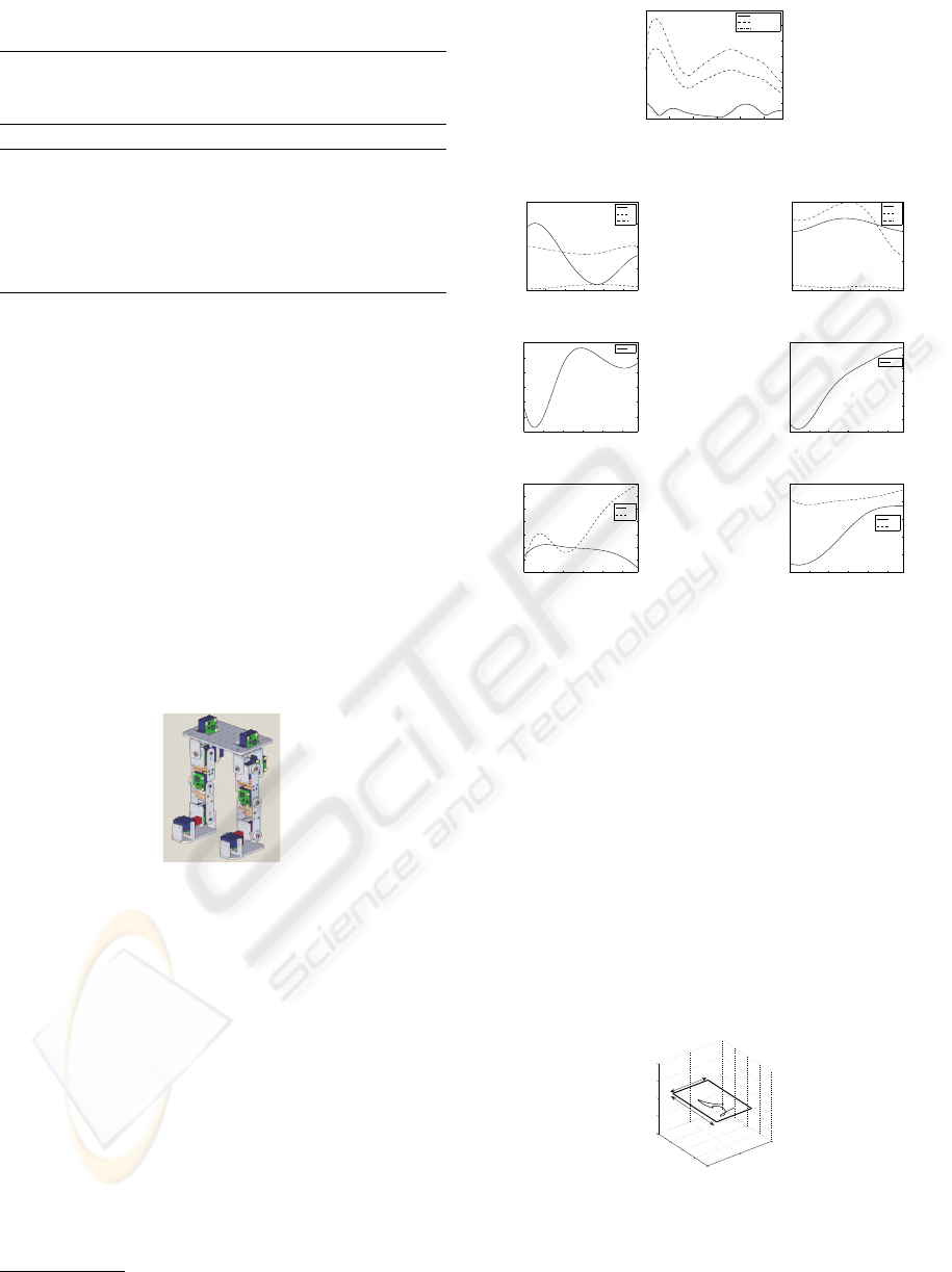
Table 2: Parameters of SPEJBL.
Physical Parameters Mass (kg) Length (m)
Torso 0.3967 d
7
= 0.140
Right Leg
Hip 0.2604 linked to torso
Thigh 0.1224 d
4
= 0.120
Shin 0.0558 d
3
= 0.120
Ankle 0.1278 d
1
= 0.042
Foot 0.3045 L
p
= 0.178
5 SIMULATION RESULTS
To validate our proposed method, we present the re-
sults of an optimal motion for the biped shown in fig-
ure 2. The desired trajectory was obtained by the op-
timization process presented in Section IV, with the
minimization of the criterion (27) satisfying the con-
straints given by (17)-(24). The figure 4 shows the
evolution of the optimal motion for a half step with
duration, of a single support, which is equal to 0.58
s. For the simulation, we use the physical parameters
of the SPEJBL
1
. The physical parameters of SPEJBL
are collected in Table 2. Figure 2 shows the photo
of SPEJBL and also the dimensional design drawn by
VariCAD software.
Figure 2: Dimensional drawing of SPEJBL.
The results shown have been obtained with T
s
=
0.58 s. The optimal motion is such that the step length
is 0.366 m and the optimal velocity is 0.6323 m/s.
These values are results of the optimization process.
The normal components of the ground reactions,
in function of time, of the stance foot during one half
step in single support are presented in figure 3. The
average vertical reaction force is 20 N, which is co-
herent with the weight of the robot which the mass
equals 2.1385 Kg. The chosen friction coefficient is
0.7.
The figure 4 shows the evolutions of joint vari-
ables q
i
(t) i = 1, ..., 12, defined by the third-order
spline function presented in Section III, in the single
1
SPEJBL is a biped robot designed in the Department of
Control Engineering of the Technical University in Prague.
0 0.1 0.2 0.3 0.4 0.5
0
5
10
15
20
25
30
35
Time [s]
Ground reaction force [N]
√(FRy
2
+FRz
2
)
µFRx
FRx
Figure 3: Normal components in the stance foot.
0 0.1 0.2 0.3 0.4 0.5
−100
−50
0
50
100
Time [s]
Position [°]
q4
q5
q6
Right hip joint positions
0 0.1 0.2 0.3 0.4 0.5
−100
−50
0
50
Time [s]
Position [°]
q7
q8
q9
Left hip joint positions
0 0.1 0.2 0.3 0.4 0.5
−60
−50
−40
−30
−20
−10
0
Time [s]
Position [°]
q3
Right knee joint position
0 0.1 0.2 0.3 0.4 0.5
10
15
20
25
30
35
40
45
Time [s]
Position [°]
q10
Left knee joint position
0 0.1 0.2 0.3 0.4 0.5
0
5
10
15
20
25
30
35
Time [s]
Position [°]
q1
q2
Right ankle joint positions
0 0.1 0.2 0.3 0.4 0.5
−40
−30
−20
−10
0
10
Time [s]
Position [°]
q11
q12
Right ankle joint positions
Figure 4: Evolution of joint positions.
support phase during one half step. Let us remark that
the evolution of each joint variable depends on the
boundary conditions ( ˙q
i,ini
, ˙q
i, fin
for i = 1,...,12 ) and
also on the intermediate configurations (q
i,int1
, q
i,int2
for i = 1,...,12 ) whose values are computed in the
optimal process.
The figure 5 shows the CoP trajectory which is al-
ways inside the support polygon determined by l
p
=
0.11 m and L
p
= 0.17 m., that is, the robot maintains
the balance during the motion. Because the minimal
distance between of CoP and the boundary of the foot
is large, smaller foot is acceptable for this cyclic mo-
tion.
−0.1
0
0.1
−0.2
−0.15
−0.1
−0.05
0
−1
−0.5
0
0.5
1
X−axis
Y−axis
Z−axis
L
P
P
l
Figure 5: The evolution of CoP trajectory.
For a set of motion velocities, the evolution of J
Γ
criterion is presented in figure 6. With respect to the
evolution of J
Γ
we can conclude that the biped robot
ICINCO 2007 - International Conference on Informatics in Control, Automation and Robotics
82

0.5 0.55 0.6 0.65 0.7 0.75
5
5.2
5.4
5.6
5.8
6
6.2
6.4
6.6
6.8
Velocity [m/s]
J [N2.m.s]
Figure 6: J
Γ
in function of several motion velocities for the
biped.
consumes more energy for low velocities to generate
one half step. Due to the limitations of the joint ve-
locities we could not obtain superior values to 0.73
m/s. The energy consumption increases probably
for higher velocity (see (Chevallereau. and Aoustin,
2001)). The robot has been designed to be able to
walk slowly, this walk require large torque and small
joint velocities. Its design is also based on large feet
in order to be able to use static walking, as a conse-
quence the feet are heavy and bulky, thus the resulting
optimal motion is close to the motion of a human with
snowshoes.
6 CONCLUSION
Optimal joint reference trajectories for the walking of
a 3D biped are found. A methodology to design such
optimal trajectories is developed. This tool is useful
to test a robot design or for the control of the robot. In
order to use classical optimization technique, the opti-
mal trajectory is described by a set of parameters: we
choose to define the evolution of the actuated relative
angle as spline functions. A cyclic solution is desired.
Thus the number of the optimization variables is re-
duced by taking into account explicitly of the cyclic
condition. Some inequality constraints such as the
limits on torque and velocity, the condition of no slid-
ing during motion and impact, some limits on the mo-
tion of the free leg are taken into account. Optimal
motion for a given duration of the step have been ob-
tained, the step length and the advance velocity are the
result of the optimization process. The result obtained
are realistic with respect to the size of the robot under
study. Optimal motion for a given motion velocity
can also be studied, in this case the motion velocity is
consider as a constraint. The proposed method to de-
fine optimal motion will be tested on other prototype
with dimension closer to human.
REFERENCES
Beletskii, V. V. and Chudinov, P. S. (1977). Parametric
optimization in the problem of bipedal locomotion.
Izv. An SSSR. Mekhanika Tverdogo Tela [Mechanics
of Solids], (1):25–35.
Bessonnet, G., Chesse, S., andSardin, P. (2002). Generating
optimal gait of a human-sized biped robot. In Proc.
of the fifth International Conference on Climbing and
Walking Robots, pages 717–724.
Channon, P. H., Hopkins, S. H., and Pham, D. T. (1992).
Derivation of optimal walking motions for a bipedal
walking robot. Robotica, 2(165–172).
Chevallereau., C. and Aoustin, Y. (2001). Optimal refer-
ence trajectories for walking and running of a biped.
Robotica, 19(5):557–569.
Formal’sky, A. (1982). Locomotion of Anthropomorphic
Mechanisms. Nauka, Moscow [In Russian].
Grishin, A. A., Formal’sky, A. M., Lensky, A. V., and Zhit-
omirsky, S. V. (1994). Dynamic walking of a vehicle
with two telescopic legs controlled by two drives. Int.
J. of Robotics Research, 13(2):137–147.
Khalil, W. and Dombre, E. (2002). Modeling, identification
and control of robots. Hermes Sciences Europe.
L. Hu, C. Z. and Sun, Z. (2006). Biped gait optimization us-
ing spline function based probability model. in Proc.
of the IEEE Conference on Robotics and Automation,
pages 830–835.
M. Sakaguchi, J. Furushu, A. S. and Koizumi, E. (1995).
A realization of bunce gait in a quadruped robot with
articular-joint-type legs. Proc. of the IEEE Conference
on Robotics and Automation, pages 697–702.
Miossec, S. and Aoustin, Y. (2006). Dynamical synthesis of
a walking cyclic gait for a biped with point feet. Spe-
cial issue of lecture Notes in Control and information
Sciences, Ed. Morari, Springer-Verlag.
M.W.Walker and D.E.Orin (1982). Efficient dynamic com-
puter simulation of robotics mechanism. Trans. of
ASME, J. of Dynamic Systems, Measurement and
Control, 104:205–211.
Rostami, M. and Besonnet, G. (1998). Impactless sag-
ital gait of a biped robot during the single support
phase. In Proceedings of International Conference on
Robotics and Automation, pages 1385–1391.
Roussel, L., de Wit, C. C., and Goswami, A. (2003). Gener-
ation of energy optimal complete gait cycles for biped.
In Proc. of the IEEE Conf. on Robotics and Automa-
tion, pages 2036–2042.
Saidouni, T. and Bessonnet, G. (2003). Generating globally
optimised saggital gait cycles of a biped robot. Robot-
ica, 21(2):199–210.
Vukobratovic, M. and Stepanenko, Y. (1972). On the stabil-
ity of anthropomorphic systems. Mathematical Bio-
sciences, 15:1–37.
Zonfrilli, F., Oriolo, M., and Nardi, T. (2002). A biped loco-
motion strategy for the quadruped robot sony ers-210.
In Proc. of the IEEE Conf. on Robotics and Automa-
tion, pages 2768–2774.
MODELING AND OPTIMAL TRAJECTORY PLANNING OF A BIPED ROBOT USING NEWTON-EULER
FORMULATION
83
