
BAYESIAN ADAPTIVE SAMPLING FOR BIOMASS
ESTIMATION WITH QUANTIFIABLE UNCERTAINTY
Pinky Thakkar
Department of Computer Engineering, San Jose State University, San Jose, CA 95192, USA
Steven M. Crunk, Marian Hofer, Gabriel Cadden, Shikha Naik
Department of Mathematics, San Jose State University, San Jose, CA 95192, USA
Kim T. Ninh
Department of Computer Engineering, San Jose State University, San Jose, CA 95192, USA
Keywords: Adaptive Sampling, Bayesian Inference, BRDF, Maximum Entropy, Optimal Location Selection.
Abstract: Traditional methods of data collection are often expensive and time consuming. We propose a novel data
collection technique, called Bayesian Adaptive Sampling (BAS), which enables us to capture maximum
information from minimal sample size. In this technique, the information available at any given point is
used to direct future data collection from locations that are likely to provide the most useful observations in
terms of gaining the most accuracy in the estimation of quantities of interest. We apply this approach to the
problem of estimating the amount of carbon sequestered by trees. Data may be collected by an autonomous
helicopter with onboard instrumentation and computing capability, which after taking measurements, would
then analyze the currently available data and determine the next best informative location at which a
measurement should be taken. We quantify the errors in estimation, and work towards achieving maximal
information from minimal sample sizes. We conclude by presenting experimental results that suggest our
approach towards biomass estimation is more accurate and efficient as compared to random sampling.
1 INTRODUCTION
Bayesian Adaptive Sampling (BAS) is a
methodology which allows a system to examine
currently available data in order to determine new
locations at which to take new readings. This
procedure leads to the identification of locations
where new observations are likely to yield the most
information about a process, thus minimizing the
required data that must be collected. As an example
of the application of this methodology, we examine
the question of standing woods in the United States.
In order to estimate the amount of carbon
sequestered by trees in the United States, the amount
of standing woods must be estimated with
quantifiable uncertainty (Wheeler, 2006). Such
estimates come from either satellite images or near
ground measurements. The amounts of error in the
estimates from these two approaches are currently
unknown. To this end, an autonomous helicopter
with differential GPS (Global Positioning System),
LIDAR (Light Detection and Ranging), stereo
imagers, and spectrometers has been developed as a
testing platform for conducting further studies
(Wheeler, 2006). These instruments are capable of
measuring the reflectance data and the location of
the Sun and helicopter in terms of the zenith and the
azimuth angles (Figure 1). The objective is to
develop a controlling software system for this
robotic helicopter, which optimizes the required
ground sampling.
The first simplistic data collection method is to
conduct an exhaustive ground sampling i.e. to send
the helicopter to every possible location. The second
approach is to perform random sampling until the
estimates have acceptable standard errors. Although
random sampling presents a possibility that the
229
Thakkar P., M. Crunk S., Hofer M., Cadden G., Naik S. and T. Ninh K. (2007).
BAYESIAN ADAPTIVE SAMPLING FOR BIOMASS ESTIMATION WITH QUANTIFIABLE UNCERTAINTY.
In Proceedings of the Fourth International Conference on Informatics in Control, Automation and Robotics, pages 229-236
DOI: 10.5220/0001628702290236
Copyright
c
SciTePress

helicopter will take samples from the locations that
offer the greatest amount of information and
therefore reduce the needed sample size, there is no
guarantee that such a sample set will be chosen
every time. The third and more efficient method is to
take only a few samples from “key” locations that
are expected to offer the greatest amount of
information. The focus of this paper is to develop a
methodology that will identify such key locations
from which the helicopter should gather data.
Figure 1: θ
S
, φ
S
are the zenith and the azimuth angles of
the Sun, and θ
V
, φ
V
are the zenith and the azimuth angles
of the view, respectively (Wheeler, 2006).
In the work described here, the key locations are
identified using current and previously collected
data. The software works in tandem with the
sampling hardware to control the helicopter’s
position. Once a sample has been taken, the data are
fed into the system, which then calculates the next
best location to gather further data. Initially, the
system assumes an empirical model for the ground
being examined. With each addition of data from the
instruments, the parameter estimates of the model
are updated, and the BAS methodology is used to
calculate the helicopter’s next position. This process
is repeated until the estimated uncertainties of the
parameters are within a satisfactory range. This
method allows the system to be adaptive during the
sampling process and ensures adequate ground
coverage.
The methodology employs a bi-directional
reflectance distribution function (BRDF), in which
the calculation of the amount of reflection is based
on the observed reflectance values of the object, and
the positions of the Sun and the viewer (Nicodemus,
1970). The advantage of using this function is that it
enables the system to compensate for different
positions of the Sun during sampling. Once the
reflectance parameters are estimated, BAS uses the
principle of maximum entropy to identify the next
location where new observations are likely to yield
the most information.
In summary, the BAS methodology allows the
system to examine currently available data with
regards to previously collected data in order to
determine new locations at which to take new
reflectance readings. This procedure leads to the
identification of locations where new observations
are likely to yield the most information.
2 RELATED WORK
Computing view points based on maximum entropy
using prior information has been demonstrated by
Arbel et al., 1970. They used this technique to create
entropy maps for object recognition. Vazquez et al.,
2001 also demonstrated a technique for computing
good viewpoints; however their research was based
on Information Theory. Whaite et al., 1994
developed an autonomous explorer that seeks out
those locations that give maximum information
without using a priori knowledge of the
environment. Makay, 1992 used Shannon’s entropy
to obtain optimal sample points that would yield
maximum information. The sample points are taken
from the locations that have largest error bars on the
interpolation function. In our work, the optimal
locations that offer maximum amount of information
are identified using the principle of maximum
entropy, where the maximization is performed using
techniques suggested by Sebastiani et al., 2000.
3 MODEL
The model for the data used in our framework is
based on the semi-empirical MISR (multi-angle
imaging spectrometer) BRDF Rahman model
(Rahman et al., 1993):
[]
()
1
(,,,)
cos( ) cos( ){cos( ) cos( )}
exp ( ) ( , , , )
svsv
k
sv s v
svsv
r
bp h
θ
θφφ
ρθ θ θ θ
θθφφ
−
=
+⋅
−⋅ Ω ⋅
(1)
where
1
(,,,)1
1(,,,)
svsv
s
vsv
h
G
ρ
θθφφ
θ
θφφ
−
=+
+
(2)
ICINCO 2007 - International Conference on Informatics in Control, Automation and Robotics
230

)cos()tan()tan(2)(tan)(tan
),,,(
22
vsvsvs
vsvs
G
φφθθθθ
φ
φ
θ
θ
−−+
=
(3)
)cos()sin()sin()cos()cos()(
vsvsvs
p
φ
φ
θ
θ
θ
θ
−
+=Ω
(4)
where
),,,(
vsvs
r
φ
φ
θ
θ
is the measured reflectance,
ρ
is the surface reflectance at zenith, k is the
surface slope of reflectance,
b is a constant
associated with the hotspot, or "antisolar point" (the
point of maximum reflectivity, which is the position
where the sensor is in direct alignment between the
Sun and the ground target),
ss
φ
θ
, are the zenith and
the azimuth angles of the Sun, respectively (Figure
1), and
vv
φ
θ
, are the zenith and the azimuth angles
of the view, respectively (Figure 1).
4 METHODOLOGY
Our framework consists of the following two steps:
1. Parameter Estimation: In this step, we
estimate the values of the parameters (
ρ
,
k and b ), and their covariance matrix and
standard errors, given the data collected to
date of the amount of observed reflected
light, and the zenith and azimuth angles of
the Sun and the observer.
2. Bayesian Adaptive Sampling (Optimal
Location Identification): In this step, we
use the principle of maximum entropy to
identify the key locations from which to
collect the data.
Once the key location is identified, the helicopter
goes to that location and the instruments on the
helicopter measure the reflectance information. This
information is then fed into the Parameter
Estimation stage and the new values of the
parameters (
ρ
, k and b ) are calculated. This
process is repeated until the standard errors of the
parameters achieve some predefined small value,
ensuring adequacy of the estimated parameters
(Figure 2).
5 IMPLEMENTATION
5.1 Parameter Estimation
The input to this module is the observed reflectance
value (r), zenith and azimuth angles of the Sun
),(
ss
φ
θ
, and zenith and azimuth angles of the
observer
),(
vv
φ
θ
. The parameters (
ρ
, k and b )
are estimated using the following iterated linear
regression algorithm:
First, a near linear version of this model is
accomplished by taking the natural logarithm of
),,,(
vsvs
r
φ
φ
θ
θ
, which results in the following
Figure 2: Overview of Bayesian Adaptive Sampling.
BAYESIAN ADAPTIVE SAMPLING FOR BIOMASS ESTIMATION WITH QUANTIFIABLE UNCERTAINTY
231

equation:
[]
),,,(ln)(.
)}cos()){cos(cos()cos(ln
)1(ln),,,(ln
vsvs
vsvs
vsvs
hpb
kr
φφθθ
θθθθ
ρ
φ
φ
θ
θ
+Ω−
+
⋅−+=
(5)
Note that aside from the term
),,,(ln
vsvs
h
φ
φ
θ
θ
, which contains a nonlinear
ρ
, the function ln(r) is linear in all three
parameters,
)ln(
ρ
, k , and b . “Linearization” of
)ln(h is accomplished by using the value of
ρ
from the previous iteration, where at iteration n in
the linear least-squares fit
),,,(
vsvs
h
φ
φ
θ
θ
is taken
to be the constant
),,,(1
1
1),,,(
)1(
)(
vsvs
n
vsvs
n
G
h
φφθθ
ρ
φφθθ
+
−
+=
−
(6)
where
)0(
ρ
is set equal to zero.
Second, regression is performed on our linearized
model to calculate the estimates of the following
quantities:
•
ρ
, k and b , the parameters
•
1−
R
, covariance matrix of the estimated
parameters (
ρ
, k and b )
•
σ
, the standard deviation of the errors,
(which are assumed to be independent
identically distributed random variables from
a normal distribution with zero mean)
Third, the current estimated value of
ρ
is then
used in
),,,(
vsvs
h
φ
φ
θ
θ
, and regression is again
performed.
This procedure is repeated until the estimate
of
ρ
converges.
5.2 Bayesian Adaptive Sampling
This module identifies the best informative location
),(
vv
φ
θ
to which to send the helicopter. We employ
the principle of maximum entropy, in which the
available information is analyzed in order to
determine a unique epistemic probability
distribution. The maximization is performed as per
techniques suggested by Sebastiani et al., 2000,
where in order to maximize the amount of
information about the posterior parameters, we
should maximize the entropy of the distribution
function. Mathematically, maximizing the entropy is
achieved by maximizing
1
log[ ( ) ]XXR
−
′
Σ+
(7)
where ∑ is covariance matrix of the error terms,
1−
R
is covariance matrix of the estimates of the
parameter
ρ
, k and b , and X is matrix of input
variables where each row in X is associated with one
observation
[
]
21
1 xxX
=
(8)
where
[]
)}cos()){cos(cos()cos(ln
1
vsvs
x
θθθθ
+
=
)cos()sin()sin(
)cos()cos()(
2
vsvs
vs
px
φφθθ
θ
θ
−+
−
=
Ω
=
Under the assumption that the errors are
independent normally distributed random variables
with mean zero and variance
2
σ
, (7) reduces to
maximizing
(
)
12
/1
−
′
+
XRXI
σ
. (9)
Note that
2
σ
and
1−
R
are estimated in module 1
and are thus at this stage assumed to be known
quantities. The matrix X contains both past
observations, in which case all elements of each
such row of X are known, and one or more new
observations where the zenith and the azimuth
angles of the Sun
),(
ss
φ
θ
are known, so the only
remaining unknown quantities in (9) are the values
of
v
θ
and
v
φ
(the zenith and azimuth angles of the
helicopter viewpoint) in rows associated with new
observations. Thus, the new location(s) to which the
helicopter will be sent are the values of
v
θ
and
v
φ
in rows of X associated with new observations that
maximize (9).
ICINCO 2007 - International Conference on Informatics in Control, Automation and Robotics
232

6 EXPERIMENT
We conduct two simulated experiments in which the
estimates of the model parameters are calculated. In
the first experiment, “Estimation Using Random
Observations”, the data is collected by sending the
helicopter to random locations. In the second
experiment, “Estimation using BAS”, the data is
collected using BAS.
The experiments are conducted under the
following assumptions:
• The view zenith angle (
v
θ
) is between 0 and
2/
π
, and the view azimuth angle (
v
φ
) is
between 0 and 2
π
( ≈ 6.283185).
• The Sun moves 2
π
radians in a 24-hour
period, i.e., at the rate of slightly less then
0.005 radians per minute.
• It takes about 2 minutes for the helicopter to
move to a new location. Thus, the position of
the Sun changes approximately 0.01 radians
between measurements.
In our simulation, the true values of the
parameters
ρ
,
k
and
b
are 0.1, 0.9, and -0.1,
respectively. For the purpose of this paper, the
observed values were simulated with added noise
from the process with known parameters. This
allows us to measure the efficacy of the algorithm in
minimizing the standard errors of the parameter
estimates, and also the estimates of the parameters.
In actual practice, the parameters would be
unknown, and we would have no way of knowing
how close our estimates are to the truth, that is, if the
estimates are as accurate as implied by the error
bars.
6.1 Estimation using Random
Observations
In this experiment, we send the helicopter to 20
random locations to collect data. Starting with the
fifth observation, we use the regression-fitting
algorithm on the collected input data set (the
observed reflectance information, and the positions
of the Sun and the helicopter), to estimate the values
of the parameters
ρ
,
k
,
b
as well as their standard
errors. Table 1 shows the results of this experiment
6.2 Estimation using BAS
In this experiment, the first five locations of the
helicopter are chosen simultaneously using an
uninformative prior distribution (i.e., as no estimate
of
1−
R
has yet been formed; it is taken to be
I
2
σ
)
and an X matrix with five rows in which the position
of the Sun
),(
ss
φ
θ
is known and (9) is maximized
over five pairs of helicopter viewpoints
v
θ
and
v
φ
.
Subsequently, we use BAS to calculate the next
best informative location for the helicopter to move
to in order to take a new reflectance observation., in
which case the X matrix contains rows associated
with previous observations, and (9) is maximized
over a single new row of the X matrix in which the
position of the Sun
),(
ss
φ
θ
is known and the only
unknowns are a single pair of helicopter viewpoint
values,
v
θ
and
v
φ
, in the last row of the X matrix.
Table 2 shows the results from this experiment.
In both experiments, estimates of the parameters,
along with their standard errors, cannot be formed
until at least five observations have been taken.
7 RESULTS
In this section, we compare and analyze the results
of our two experiments. The comparison results
(Figure 3, Figure 4 and Figure 5) show that the
estimates using the data from the "well chosen"
locations using BAS are closer to the true values,
1.
=
ρ
,
9.0
=
k
and
1.0
−
=
b
, than the estimates based
on data from the randomly chosen locations. Also,
the error bars using BAS are much shorter indicating
higher confidence in the estimates of the parameters
based on the "well chosen locations", i.e., the length
of the error bar for the estimate calculated using
data/observations from five well chosen locations is
as short as the error bar based on data collected from
20 random locations.
Within each figure (Figure 3, Figure 4 and Figure
5), the horizontal axis indicates the number of
observations between five and twenty that were used
in forming the estimates. The vertical axis is on the
scale of the parameter being estimated. Above each
observation number, an "o" represents the estimate
(using the data from the first observation through the
observation number under consideration) of the
parameter using the randomly chosen locations and
the observations from those locations. The "x"
represents the estimate of the parameter using
observations taken at locations chosen through BAS.
BAYESIAN ADAPTIVE SAMPLING FOR BIOMASS ESTIMATION WITH QUANTIFIABLE UNCERTAINTY
233
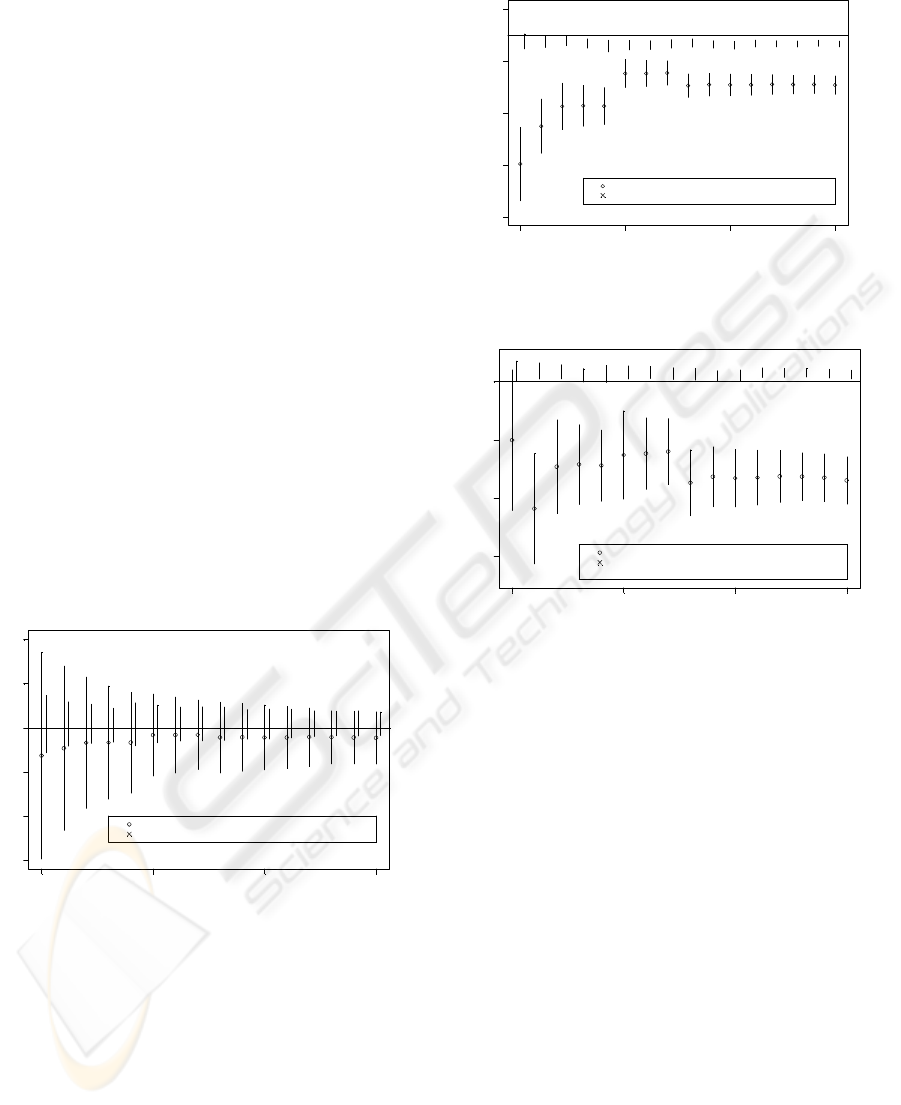
The error bars are the standard errors of the
estimated parameter based on these observations
taken at "well chosen locations". The "bar" is the
error bar, which extends one standard error above
and below the parameter estimate. The horizontal
line represents the true value of the parameter in our
simulation.
Note that in Figure 4 and Figure 5, the error bars
rarely overlap the true value of the parameter. This
can be attributed to two factors. In large part, this is
due to the fact that they are "error bars" with a
length of one standard error beyond the point
estimate. Traditional 95% statistical confidence
intervals based on two standard errors would in
virtually every case overlap the true values.
Additionally, these are cumulative plots, in which
the same data is used, adding observations to form
the parameter estimates as one moves to the right in
each figure. Thus the point estimates and error bars
are dependent upon one another within a figure.
Finally, we see that the estimates using BAS (to
select the points from which to take observation) are
generally closer to the truth than when we use
random points to take observations, and more
importantly the standard errors associated with any
given number of observations are much smaller.
Number of included observations
5 101520
-0.05 0.0 0.05 0.10 0.15 0.20
ρ
Using random locations to take observations
Using locations identified by BAS to take observations
x
x
x
x
x
x
x
x
x
x
x
x
x
x
x
x
Figure 3: Estimates and error bars for
ρ
.
Number of included observations
b
5 101520
-0.8 -0.6 -0.4 -0.2 0.0
Using random locations to take observations
Using locations identified by BAS to take observations
x
x
x
x
x
x
x
x
x
x
x
x
x
x
x
x
Figure 4: Estimates and error bars for
b
.
Number of included observations
k
5101520
0.75 0.80 0.85 0.90
Using random locations to take observations
Using locations identified by BAS to take observations
x
x
x
x
x
xx
x
x
x
x
x
x
x
x
x
Figure 5: Estimates and error bars for
k
.
8 CONCLUSION
Our initial results have shown that BAS is highly
efficient compared to random sampling. The rate at
which the standard errors, or the error bars, are
reduced is much quicker, and hence the significant
amount of information is found more quickly
compared to other traditional methods. We have also
shown that this methodology performs well even in
the absence of any preliminary data points. Further
simulation has shown evidence that BAS can be
three times as efficient as random sampling. This
efficiency amounts to savings of time and money
during actual data collection and analysis.
In addition to the application discussed in this
paper, the theoretical framework presented here is
generic and can be applied directly to other
applications, such as, military, medical, computer
vision, and robotics.
Our proposed framework is based on the
ICINCO 2007 - International Conference on Informatics in Control, Automation and Robotics
234

multivariate normal distribution. The immediate
extensions of this framework will be:
a) To accommodate non-normal parameter
estimate distributions. As part of our future study,
we intend to employ sampling methodologies using
Bayesian Estimation Methods for non-normal
parameter estimate distributions. and
b) To use cost effectiveness as an additional
variable. In this initial work, the focus was to
identify the viewpoints that would give us the most
information. However, it is not always feasible or
efficient to send the helicopter to this next “best”
location. As part of our future work, we intend to
identify the next “best efficient” location for the
helicopter from which it should collect data.
ACKNOWLEDGEMENTS
This work was done as part of the CAMCOS (Center
for Applied Mathematics, Computation, and
Statistics) student industrial research program in the
Department of Mathematics at San Jose State
University.
This work was supported in part by the NASA
Ames Research Center under Grant NNA05CV42A.
We are appreciative of the help of Kevin Wheeler,
Kevin Knuth and Pat Castle, who while at Ames
suggested these research ideas and provided
background materials.
REFERENCES
Arbel, T., Ferrie, F., “Viewpoint selection by navigation
through entropy maps,” in Proc. 7th IEEE Int. Conf.
on Computer Vision, Greece, 1999, pp. 248–254
MacKay, D., “A clustering technique for digital
communications channel equalization using radial
basis function networks,” Neural Computation, vol.4,
no.4, pp. 590–604, 1992.
Nicodemus, F. E., “Reflectance Nomenclature and
Directional Reflectance and Emissivity,” in Applied
Optics, vol. 9, no. 6, June 1970, pp. 1474-1475.
Rahman, H. B., Pinty, B., Verstaete, M. M., “A coupled
surface-atmosphere reflectance (CSAR) model. Part 1:
Model description and inversion on synthetic data,”
Journal of Geophysical Research, vol.98, no.4, pp.
20779–20789, 1993.
Sebastiani P., Wynn, H. P., “Maximum entropy sampling
and optimal Bayesian experimental design,” Journal of
Geophysical Research, 62, Part1, pp. 145-157, 2000.
Sebastiani, P., and Wynn, H. P.
“Experimental Design to Maximize Information,”
Bayesian Inference and Maximum Entropy Methods
in Science and Engineering: 20th Int. Workshop. AIP
Conf. Proc., Gif sur Yvette, France, vol. 568, pp 192-
203, 2000.
Vazquez, P. Feixas, P., Sbert, M., M., Heidrich, W.,
“Viewpoint selection using viewpoint entropy,” in
Proc. of Vision, Modeling, and Visualization,
Germany, 2001, pp. 273–280.
Whaite, P., Ferrie, F. P., “Autonomous exploration:
Driven by uncertainty,” in Proc. of the Conf. On on
Computer Vision and Pattern Recognition, California,
1994, pp. 339–346.
Wheeler, K. R., "Parameterization of the Bidirectional
Surface Reflectance," NASA Ames Research Center,
MS 259-1, unpublished.
BAYESIAN ADAPTIVE SAMPLING FOR BIOMASS ESTIMATION WITH QUANTIFIABLE UNCERTAINTY
235

Table 1: Observation and Estimates Using Random Sampling.
Table 2: Observations and Estimates using BAS.
Observation
Number
v
θ
v
φ
r
Estimate (se)
of
ρ
Estimate (se) of
k
Estimate (se) of
b
1 0.460 0.795 0.172364
2 0.470 0.805 0.177412
3 1.561 3.957 0.161359
4 1.561 0.825 0.183571
5 1.265 3.977 0.129712 0.1041 (0.0325) 0.90904 (0.00879) -0.1249 (0.0290)
6 0.514 0.845 0.173072 0.1042 (0.0252) 0.90927 (0.00700) -0.1255 (0.0233)
7 1.561 3.400 0.160130 0.1045 (0.0223) 0.90857 (0.00615) -0.1220 (0.0199)
8 1.172 4.007 0.130101 0.1029 (0.0192) 0.90547 (0.00577) -0.1329 (0.0180)
9 0.723 0.875 0.189697 0.1039 (0.0244) 0.90663 (0.00748) -0.1428 (0.0228)
10 1.561 0.885 0.192543 0.1042 (0.0213) 0.90801 (0.00569) -0.1394 (0.0185)
11 0.527 0.895 0.172811 0.1042 (0.0193) 0.90796 (0.00523) -0.1392 (0.0172)
12 1.561 4.047 0.164530 0.1044 (0.0193) 0.90696 (0.00519) -0.1343 (0.0167)
13 1.561 4.057 0.164822 0.1046 (0.0190) 0.90636 (0.00505) -0.1314 (0.0161)
14 1.137 4.067 0.131443 0.1038 (0.0169) 0.90483 (0.00471) -0.1365 (0.0148)
15 0.713 0.935 0.183894 0.1042 (0.0169) 0.90538 (0.00480) -0.1397 (0.0149)
16 1.561 0.945 0.192280 0.1048 (0.0163) 0.90777 (0.00427) -0.1333 (0.0136)
17 1.187 4.097 0.134701 0.1047 (0.0146) 0.90757 (0.00399) -0.1340 (0.0125)
18 0.655 0.965 0.176841 0.1048 (0.0140) 0.90779 (0.00385) -0.1349 (0.0120)
19 1.561 4.117 0.168819 0.1049 (0.0142) 0.90694 (0.00388) -0.1321 (0.0120)
20 1.148 4.127 0.132199 0.1045 (0.0132) 0.90617 (0.00373) -0.1349 (0.0114)
Observation
Number
v
θ
v
φ
r
Estimate (se)
of
ρ
Estimate (se)
of
k
Estimate (se) of
b
1 0.114 1.673 0.157552
2 0.882 6.013 0.156616
3 0.761 0.917 0.192889
4 0.678 1.308 0.180404
5 0.260 0.114 0.152558 0.0683 (0.1172) 0.8497 (0.0607) -0.5958 (0.1413)
6 1.195 2.367 0.146659 0.0767 (0.0932) 0.7906 (0.0476) -0.4506 (0.1040)
7 0.237 2.805 0.149475 0.0830 (0.0746) 0.8268 (0.0404) -0.3745 (0.0893)
8 0.166 1.700 0.155497 0.0832 (0.0641) 0.8286 (0.0345) -0.3722 (0.0788)
9 0.320 2.012 0.154191 0.0831 (0.0572) 0.8277 (0.0307) -0.3735 (0.0713)
10 1.224 4.085 0.129133 0.0917 (0.0465) 0.8369 (0.0381) -0.2483 (0.0539)
11 1.409 3.442 0.135005 0.0917 (0.0431) 0.8380 (0.0309) -0.2481 (0.0503)
12 0.092 1.559 0.154096 0.0920 (0.0394) 0.8398 (0.0285) -0.2462 (0.0471)
13 0.806 0.891 0.200401 0.0888 (0.0402) 0.8129 (0.0284) -0.2952 (0.0453)
14 1.256 5.467 0.147654 0.0891 (0.0385) 0.8181 (0.0259) -0.2914 (0.0433)
15 0.227 1.284 0.155373 0.0889 (0.0368) 0.8169 (0.0248) -0.2919 (0.0418)
16 1.129 5.522 0.148721 0.0889 (0.0354) 0.8174 (0.0236) -0.2918 (0.0402)
17 0.507 5.696 0.150381 0.0891 (0.0333) 0.8183 (0.0225) -0.2904 (0.0380)
18 0.119 4.363 0.142232 0.0890 (0.0302) 0.8181 (0.0207) -0.2908 (0.0357)
19 0.245 0.524 0.151915 0.0889 (0.0299) 0.8172 (0.0205) -0.2901 (0.0355)
20 0.446 2.408 0.144471 0.0884 (0.0297) 0.8149 (0.0204) -0.2930 (0.0354)
ICINCO 2007 - International Conference on Informatics in Control, Automation and Robotics
236
