IRREVERSIBILITY MODELING APPLIED TO THE CONTROL

OF COMPLEX ROBOTIC DRIVE CHAINS

Omar Al Assad, Emmanuel Godoy

Ecole Supérieure d’Electricité (Supélec) Gif-sur-Yvette F-91192 Cedex, France

Vincent Croulard

General Electric Healthcare, 283 rue de la Minière, Buc F-78530 Cedex, France

Keywords: Robotic, Modeling, Drive chain, Mechanical irreversibility, Efficiency, Gearbox.

Abstract: The phenomena of static and dry friction may lead to difficult problems during low speed motion (e.g. stick

slip phenomenon). However, they can be used to obtain irreversible mechanical transmissions. The latter

tend to be very hard to model theoretically. In this paper, we propose a pragmatic approach to model

irreversibility in robotic drive chains. The proposed methodology consists of using a state machine to

describe the functional state of the transmission. After that, for each state we define the efficiency

coefficient of the drive chain. This technique gives conclusive results during experimental validation and

allows reproducing a reliable robot simulator. This simulator is set up for the purpose of position control of

a medical positioning robot.

1 INTRODUCTION

Modern control theories in robotics are more and

more turned towards model-based controllers such as

computed torque controllers, adaptive controllers or

feedforward dynamics compensators. Therefore,

dynamic modeling has become an inevitable step

during controllers design. Besides, accurate dynamic

modeling is a key point during simulations and the

mechanism design process.

In the literature, the problem of robot dynamic

odeling is treated in two steps. The first one

concerns the mechanical behavior of the robot

external structure considered often as a rigid

structure. Many researchers have treated this

problem and different techniques have been

introduced to solve this issue. The two best-known

methods in this matter are the Newton-Euler

formulation and the Lagrange formulation (Khalil,

1999). The second step concerns the drive chain

modeling which includes motors, gears and power

loss modeling. Despite the advances made in the

field of mechanical modeling, some issues are still

without a convenient solution. We can mention, for

instance, the phenomenon of irreversibility that

characterizes certain types of mechanical

transmissions such as worm gears (Henriot, 1991).

This characteristic is often required for security

reasons like locking the joint in case of motor failure

or unexpected current cut-off. The purpose of this

paper is to present a new modeling approach based

on a state machine in order to simulate irreversible

transmissions.

This paper is organized as follows. In section 2,

give a brief overview of the LCA vascular robot,

which is used as an application for this study.

Section 3 presents details about the modeling

approach used for the robot structure and drive chain.

Section 4 presents the irreversibility modeling issue

and the proposed solution. Section 5 illustrates the

experimental validation results. Finally, section 7

presents some concluding remarks.

2 LCA ROBOT PRESENTATION

The LCA vascular robot (figure 1) is used for

medical X-ray imaging. It is a four-degrees-of-

freedom open-chain robot composed of the following

links: the L-arm (rotational joint), the Pivot

(rotational joint), the C-arc (it has a translation

movement in a circular trajectory template. Hence, it

217

Al Assad O., Godoy E. and Croulard V. (2007).

IRREVERSIBILITY MODELING APPLIED TO THE CONTROL OF COMPLEX ROBOTIC DRIVE CHAINS.

In Proceedings of the Fourth International Conference on Informatics in Control, Automation and Robotics, pages 217-222

DOI: 10.5220/0001629802170222

 SciTePress

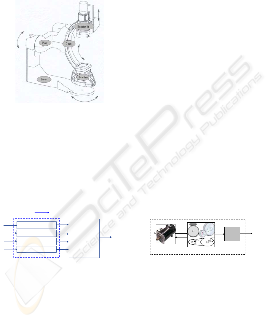
can be considered as a rotational joint around the

virtual axis crossing the C-arc center) and the Lift

(prismatic joint)

Figure 1: LCA robot.

3 MODELING APPROACH

The modeling of the LCA robot requires a clear

distinction between the dynamic model of the

mechanical structure and the drive chain model

(figure 2). In fact, the dynamic model describes

merely the relation between the applied torques and

the ideal mechanical reaction of the gantry given by

the joints acceleration.

The drive chain model takes into account the hard

nonlinearities of the system such as the joint friction

and the gear irreversibility.

L-arm Motorisation

Pivot Motorisation

C-arc Motorisation

Lift Motorisation

Robot

Dynamic

Model

Drive chain

Position

Velocity

Accelerati

Current

are the motors command voltage.

are the axes driving torques.

Figure 2: The robot model structure.

3.1 Dynamic Modeling

Two main methods can be used to calculate the

dynamic model of the robot mechanical structure.

We can mention the Newton-Euler formulation and

the Lagrange formulation (Khalil, 1999).

Most authors use the Lagrange formulation that

gives the mathematical expression of the model as:

)(),()( qQqqqCqqA +



(1)

Where are respectively the vectors of joints

position, velocity, and acceleration.

qqq



)(qA

: the 4x4 robot inertia matrix.

qqqC



⋅

),(

: the 4x1 Coriolis and centrifugal torque/

forces vector.

)(qQ

: the 4x1 gravitational torques/ forces vector.

: the 4x1 input torques/ forces vector.

To simulate the robot movement, we should use the

inverse of the dynamic model as follow:

),,( qqfq



This model can be obtained directly using the

recursive Newton-Euler equations, or it can be

inferred from equation (1):

(2)

))(),(()(

qQqqqCqAq −−Γ=

−



The “A” matrix is inverted symbolically; this will

result in a heavy mathematical expression, costly in

term of computation time. Alternatively, this inverse

can be calculated after numerical calculation

of which leads to faster simulations.

)(qA

3.2 Drive Chain Modeling

The next step consists of modeling the drive chain,

which includes the electrical motor (DC motor for

this application), the mechanical transmission (gears)

and the elements of power dissipation (friction)

(figure 3).

We will describe briefly the first and the second

elements and emphasize the third element, which is

the purpose of this paper.

gears

Motor

Friction model

Figure 3: Drive chain model.

Actually, the phenomenon of irreversibility,

obtained using specific transmissions and particular

geometric dimensioning, is a complex problem and

leads instinctively to non linear models. It can be

treated using several approaches. In a microscopic

point of view, the contacts among driving and driven

elements are modeled as well as the applied forces.

However, this rigorous approach leads to very

complex analytical models, with serious difficulties

in the implementation and simulations phases,

particularly in the case of closed loop structures

ICINCO 2007 - International Conference on Informatics in Control, Automation and Robotics

218

including controllers (Henriot, 1991). Besides, the

identification of this type of models is very

complicated due to the significant number of

parameters. In a macroscopic point of view, the

power transfer between the motor and the load is

modeled with an efficiency coefficient taking into

account the power transfer direction (load

driving/driven) (Abba, 1999), (Abba, 2003).

However, a proportional coefficient is insufficient to

represent the irreversibility behavior. In our

approach, we suggest the use of a state machine to

define the current functional state of the transmission

in order to reproduce the irreversibility.

3.2.1 DC Motor Modeling

The DC motor is a well-known electromechanical

device. Its model has two inputs, the armature

voltage and the shaft velocity. The output is the

mechanical torque applied on the shaft. The DC

motor behavior is modeled using two equations

(Pinard, 2004) the electrical equation of the armature

current (3) and the mechanical equation of the motor

torque (4):

LIREV ⋅+⋅=−

(3)

where

is the motor voltage.

is the armature

current. is the electromotive force. is

the motor velocity; and the motor parameters

are: (the back electromotive constant), (the

motor resistance) and (the motor inductance).

memf

qKE



⋅=



emf

⋅

=Γ

(4)

where is the motor torque and is the motor

torque constant ( )

emft

KK =

3.2.2 Gears Modeling

In this paper, we consider rigid gears’ models. In this

case, the model’s mathematical expression depends

only on the gear ratio N. Therefore, the output torque

is obtained using the following relation:

⋅

and the speed of the motor shaft is obtained using:

qNq



⋅=

The gear’s ratio is given by simple mathematical

expressions (Henriot, 1991) or via the gears

datasheet.

3.2.3 The Power Dissipation in Drive Chain

This section is the most essential in drive chain

modeling. In fact, good power dissipation modeling

helps to reproduce complex gear behaviors such as

irreversibility. The power dissipation will be

illustrated through the friction phenomenon.

In robotics, friction is often modeled as a function

of joint velocity. It is based on static, dry and viscous

friction (Khalil, 1999), (Abba, 2003). These models

produce accurate simulation results with simple drive

chain structures. However, in the presence of more

complex mechanisms such as worm gears these

models lack reliability.

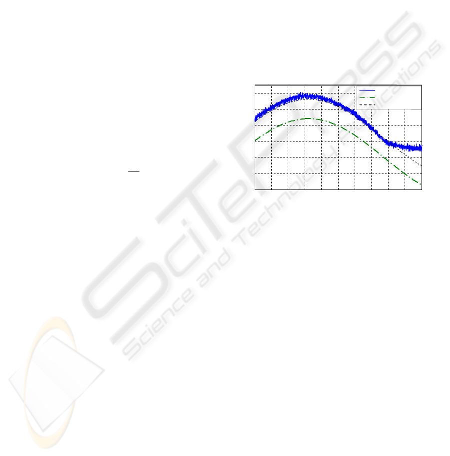
To illustrate this phenomenon, we can compare

the theoretical motor torque required to drive the

LCA pivot axis in the case of a reversible

transmission and the real measured motor torque.

Figure 4 and 5 show the applied torques on the pivot

axis during a 7°/sec and -7°/sec constant velocity

movement.

-100 -80 -60 -40 -20 0 20 40 60 80 100

-2

-1

Axis position (deg)

Torque (Nm)

Measured Tm

Load Torque

Reversible gear Tm

Figure 4: Motor and load torque variation during constant

velocity rotation (7 °/s).

During this movement, the robot dynamic is

represented by the following dynamic equation:

flm

Γ+Γ

(5)

where

is the load torque and is the friction

torque. Consequently, we expect that the motor

torque will have the same behavior as the load torque

because the friction torque is constant. However,

these results reveal an important difference between

the measured motor torque and the expected motor

torque with a drive chain using only velocity friction

model.

IRREVERSIBILITY MODELING APPLIED TO THE CONTROL OF COMPLEX ROBOTIC DRIVE CHAINS

219

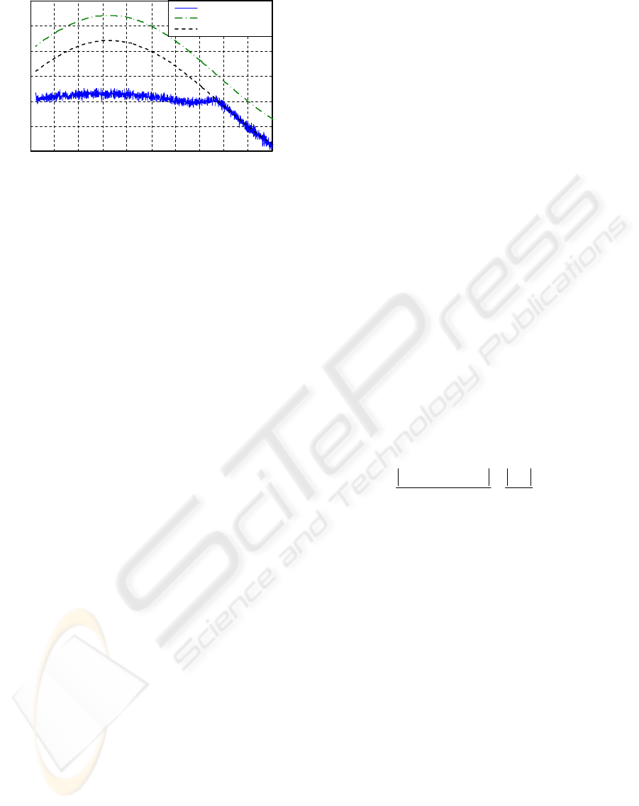
-100 -80 -60 -40 -20 0 20 40 60 80 100

-3

-2

-1

Axis position (deg)

Torque (Nm)

Reversible gear Tm

Measured Tm

Load Torque

Figure 5: Motor and load torque variation during constant

velocity rotation (-7 °/s).

We can see that the irreversibility seriously

influences the motor torque. Actually, the

irreversibility compensates the gravity torque when

the load torque becomes driving. Therefore, it is

essential to expand the friction model to take into

consideration more variables such as motor torque

and load torque in order to reproduce irreversibility

in a simulation environment. Thus, the friction model

applied on motor shaft will have the following

structure:

),,()(),(

mlmfTmfvmmfsf

qqq



ΓΓΓ+Γ+ΓΓ=Γ

(6)

where :

),(

mmfs



ΓΓ

: 4x1 vector of the static friction model

)(

mfv



: 4x1 vector of the velocity friction model

),,(

mlmfT



ΓΓΓ

: 4x1 vector of the torque friction

model.

and are the classical friction terms used

usually in drive chain modeling (Dupont, 1990),

(Armstrong, 1998). While, presents the term that

takes account of the irreversibility behavior.

limilimili

mimilimimimilimifTi

Γ⋅ΓΓ+

Γ⋅Γ

=ΓΓΓ

),,(

),,(),,(





(7)

where

),,(

milimimi



ΓΓ

and

),,(

milimili



ΓΓ

are

the motor and load friction dynamic coefficients.

Let’s consider now the complete robot dynamic

model:

flmmm

qqANqJ Γ+Γ++⋅=Γ

−



)(

(8)

where and is the 4x4

motors and gears inertia matrix. By replacing (6) in

(8) we obtain:

))(),((

qQqqqCN

+=Γ

−



llmmmfv

mmfslmmm

qqqANJ

Γ⋅+Γ⋅+Γ+

ΓΓ+Γ+⋅+=Γ

−

μμ

)(

),())((





(9)

where

and

are respectively 4x4 diagonal

matrixes:

{

}

{}

4,,1;)],,([diag

…



…



=ΓΓ=

milimilil

milimimim

μμ

By regrouping the terms of equation 11 we obtain:

(10)

)(),(

))((

mfvmmfs

llmmmm

qqANJ



Γ+ΓΓ+

Γ⋅+⋅+=Γ⋅

−

ηη

where

)(

44 mm

−

and

)(

44 ll

The new terms

and

, which depend on

and , introduce the efficiency concept in the

robot dynamic model. The next section will focus on

the proposed approach used to calculate the drive

chain efficiency coefficients.



4 EFFICIENCY COEFFICIENTS

ESTIMATION

One of the complex issues in drive chain modeling is

the estimation of the transmission efficiency

coefficient. One technique consists of theoretically

calculating the efficiency of each element of the

drive chain using the efficiency definition (Henriot,

1991):

out

Power Emitted

Power Received

(11)

The calculation of this coefficient requires the

determination of the driving element whether it is the

motor or the load. We talk then about the motor

torque efficiency (

) or the load torque efficiency

(

). Therefore, the received power “ ” could be

either from the motor or the load.

Actually, this method can be applied with simple

gear mechanisms such as spur gears, whereas for

complex gears, such as worm gears, the calculation

of the efficiency coefficient using analytical

formulas tends to be hard and inaccurate due to the

lack of information concerning friction modeling as

well as the complexity of the contact surface

between gears’ components (Henriot, 1991). The

alternative that we propose is to experimentally

identify the efficiency coefficient according to a

functional state of the drive chain, for instance, when

the load is driving the movement or when the motor

is driving the movement. This leads us to create a

state machine with the following inputs and outputs:

Table 1: State machine inputs and outputs.

ICINCO 2007 - International Conference on Informatics in Control, Automation and Robotics

220

Inputs Outputs

: motor torque (Tm)

: motor efficiency

: load torque (Tl)

: load efficiency



: motor velocity

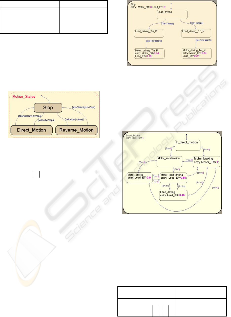
Now, we will present the states and the criteria of

states transitions that we have used for LCA robot

drive chain modeling. The state machine includes

two levels: the upper level that describes the motion

(figure 6) and the lower level that describes the

switch between motor driving and load driving states

(figures 7, 8), and associates an efficiency coefficient

for each state. In this level, the transition condition is

the sign of the velocity.

Figure 6: Motion state machine.

In the upper level, the transition condition is the

sign of the velocity. In fact, for simulation

convergence issue the drive chain is considered

stopped when

epsm

Vq <



, where is the stop

velocity threshold.

eps

In the lower level, a sub-state has been combined

to each motion state:

• The stop states (figure 7)

During the stop phase, the drive chain is

irreversible (the load torque cannot drive the

movement). Motion is observed when the motor

torque becomes superior to the load torque.

In the lower level, the state transition is based on

the motor and load torque values. As for (figure

6), represents the motor torque threshold, it is

used for simulation convergence issue

( ).

eps

Nm 10

5−

eps

Figure 7: Stop state machine.

• The direct motion states

For the direct motion state (if V>0), we have four

main states (figure 8), the states transitions are given

by the following conditions: and : the

motor is driving;

0>Γ

0<Γ

and : we distinguish

two states whether

0>Γ

or not; and : the

motor is braking (load driving)

0<Γ

Figure 8: direct motion state machine.

• The reverse motion states

The reverse motion (V<0) state machine has the

same structure as the direct motion one. We need to

replace

and

−

and . The table 1

summaries the drive chain efficiency coefficients for

each state: (Motor driving / Motor and load driving /

Load driving).

Γ−

Table 2: Drive chain efficiency coefficients.

States

Direct

motion

Reverse

motion

⋅

0.9 0.9

⋅

Γ<Γ

0.55 0.16

⋅

Γ>Γ

0.45 0.06

IRREVERSIBILITY MODELING APPLIED TO THE CONTROL OF COMPLEX ROBOTIC DRIVE CHAINS

221

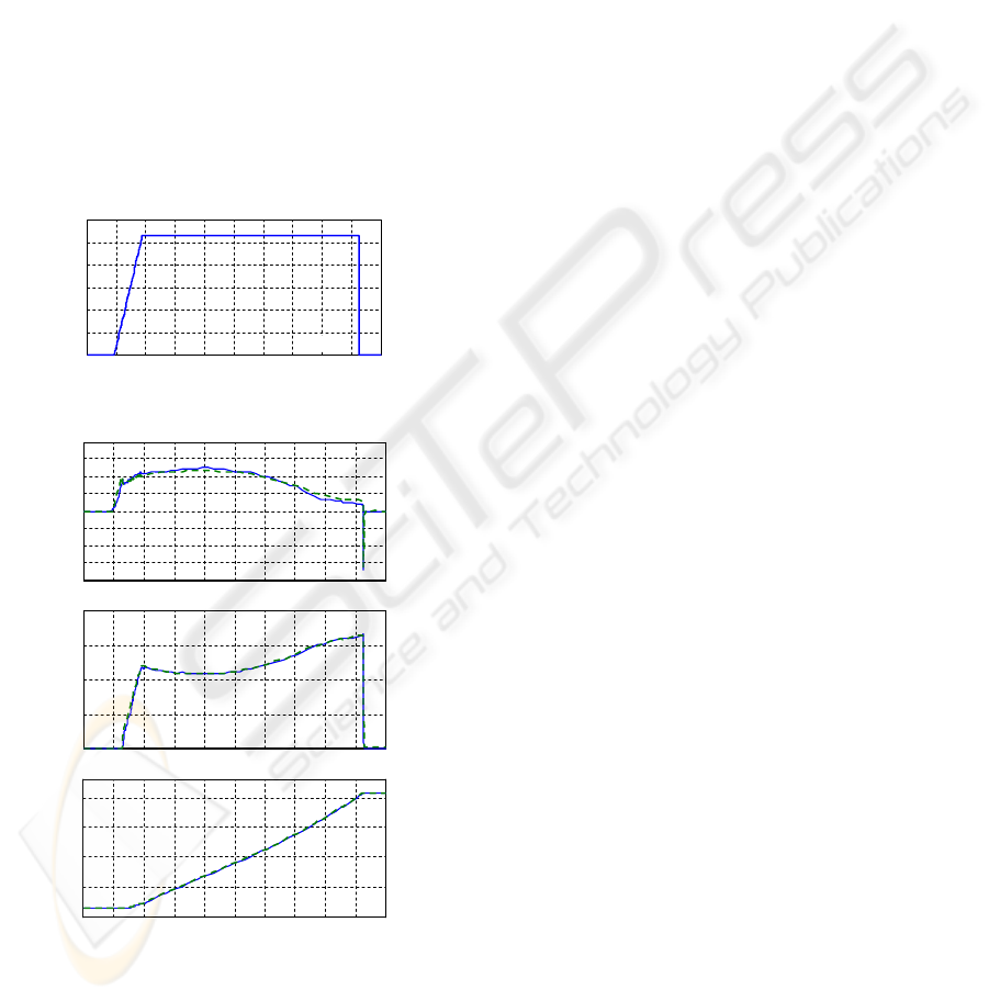
5 EXPERIMENTAL VALIDATION

The validation of the drive chain model has been

done on the pivot axis. The efficiency coefficients

have been identified using experimental measures.

We compare the open loop response of the pivot

joint and the simulation results to a voltage input for

both direct and reverse motion. Figure 9 shows the

applied voltage on the motor pivot axis for direct

motion. Figure 10 shows the experimental results

(dashed curve) of current, velocity and position and

those obtained in simulation (solid curve). We notice

in that the simulation response represents the same

behavior as the real mechanism. In this figure we

distinguish four main phases: the starting phase 24s

to 25s, the motor driving phase 25s to 37.8s, the load

driving phase 37.8s to 4.2s and the braking phase

4.2s to 4.3s.

22 24 26 28 30 32 34 36 38 40 42

Time (s)

Motor voltage (V)

Figure 9: Open loop motor command voltage.

22 24 26 28 30 32 34 36 38 40 42

-20

-15

-10

-5

Current (A)

22 24 26 28 30 32 34 36 38 40 42

Velocity (deg/sec)

22 24 26 28 30 32 34 36 38 40 42

-100

-50

100

130

Time (s)

Position (deg)

Figure 10: Direct motion outputs.

By comparing the obtained results, we notice that

the differences are low for direct motion as well as

for reverse motion. Therefore, these results prove

that the used model is able to represent accurately the

irreversibility property of the pivot drive chain.

6 CONCLUSIONS

In this paper, we presented a methodology in order to

model the irreversibility characteristic in

electromechanical drive chains. The proposed

approach uses a macroscopic modeling of the gears,

which are usually the origin of irreversibility in a

drive chains. It consists of creating a state machine

representing different functional states of the gears

and attributing an efficiency coefficient to each

specific state.

The validation of the proposed modeling was

carried out on the Pivot axis of the LCA robot. The

methodology has been tested in particular when the

position trajectory leads to some transitions “motor

driving to load driving” and the obtained results

confirm the correctness of the used model.

The perspectives of this work concern two

research orientations. The first one is the definition

and the study of an automatic procedure to identify

the efficiency coefficient for each state. The second

one is the investigation of the trajectory planning and

the control of robots with irreversible transmissions

when considering state machines for gear’s

modeling.

REFERENCES

Abba G., Chaillet N. (1999) “Robot dynamic modeling

using using a power flow approach with application to

biped locomotion”, Autonomous Robots 6, 1999, pp.

39–52.

Abba G., Sardain P.(2003), “Modélisation des frottements

dans les éléments de transmission d'un axe de robot en

vue de son identification: Friction modelling of a robot

transmission chain with identification in mind”,

Mécanique & Industries, Volume 4, Issue 4, July-

August, pp 391-396

Armstrong B. (1998), “Friction: Experimental

determination, modelling and compensation”, IEEE

International Conference on Robotics and Automation,

Philadelphia, PA, USA, April, vol. 3, pp. 1422–1427.

Dupont P.E.(1990) “Friction modeling in dynamic robot

simulation”, Robotics and Automation, 1990.

Proceedings., IEEE International Conference, pp.

1370-1376 vol.2

Henriot G. (1991) “Traité théorique et pratique des

engrenages”, 5

ed. Dunod ed. vol. 1.

Khalil W., Dombre E. (1999) “Modélisation identification

et commande des robots”, 2

ed. Hermes ed.

Pinard M. (2004), “Commande électronique des moteurs

électriques”, Paris Dunod ed. pp 157-163

ICINCO 2007 - International Conference on Informatics in Control, Automation and Robotics

222