
DESIGN OF LOW INTERACTION DISTRIBUTED DIAGNOSERS
FOR DISCRETE EVENT SYSTEMS
J. Arámburo-Lizárraga, E. López-Mellado and A. Ramírez-Treviño
CINVESTAV Unidad Guadalajara; Av. Científica 1145, Col. El Bajío; 45010 Zapopan, Jal, México
Keywords: Discrete Event Systems, Petri Nets, Distributed Diagnosis.
Abstract: This paper deals with distributed fault diagnosis of discrete event systems (DES). The approach held is
model based: an interpreted Petri net (IPN) describes both the normal and faulty behaviour of DES in which
both places and transitions may be non measurable. The diagnoser monitors the evolution of the DES
outputs according to a model that describes the normal behaviour of the DES. A method for designing a set
of distributed diagnosers is proposed; it is based on the decomposition of the DES model into reduced sub-
models which require low interaction among them; the diagnosability property is studied for the set of
resulting sub-models.
1 INTRODUCTION
Most of works study the diagnosability property and
fault detection schemes based on a centralised
approach using the global model of the DES.
Recently, fault diagnosis of DES has been addressed
through a distributed approach allowing breaking
down the complexity when dealing with large and
complex systems (Benveniste, et al., 2003; O.
Contant, et al., 2004; Debouk, et al., 2000; Genc and
Lafortune, 2003; Jiroveanu and Boel, 2003; Pencolé,
2004; Arámburo-Lizárraga, et al., 2005).
In (Debouk, et al., 2000) it is proposed a
decentralised and modular approach to perform
failure diagnosis based on Sampath's results
(Sampath, et al., 1995). In (Contant, et al., 2004) and
(Pencolé, 2004) the authors presented incremental
algorithms to perform diagnosability analysis based
on (Sampath, et al., 1995) in a distributed way; they
consider systems whose components evolve by the
occurrence of events; the parallel composition leads
to a complete system model intractable. In (Genc
and Lafortune, 2003) it is proposed a method that
handles the reachability graph of the PN model in
order to perform the analysis similarly to (Sampath,
et al., 1995); based on design considerations the
model is partitioned into two labelled PN and it is
proven that the distributed diagnosis is equivalent to
the centralised diagnosis; later, (Genc and Lafortune,
2005) extend the results to systems modelled by
several labelled PN that share places, and present an
algorithm to determine distributed diagnosis.
Our approach considers the system modelled as
an interpreted PN (IPN) allowing describing the
system with partially observable states and events;
the model includes the possible faults it may occur.
A structural characterisation and a diagnoser scheme
was presented in (Ramírez-Treviño, et al., 2004);
then in (Arámburo-Lizárraga, et al., 2005) we
proposed a methodology for designing reduced
diagnosers and presented an algorithm to split a
global model into a set of communicating sub-
models.
In this paper we present the formalisation of the
distributed system model. The proposed distributed
diagnoser scheme consists of communicating
diagnoser modules, where each diagnoser can handle
two kind of reduced models; the choice of the
reduced models depends on some considerations of
the system behaviour. In some cases the
communication between modules is not necessary.
This paper is organised as follows. In section 2
basic definitions of PN and IPN are included.
Section 3 summarises the concepts and results for
centralised diagnosis. Section 4 presents the results
related to distributed diagnosis analysis. Section V
presents the method to get reduced sub-models that
have low interaction among them.
189
Arámburo-Lizárraga J., López-Mellado E. and Ramírez-Treviño A. (2007).
DESIGN OF LOW INTERACTION DISTRIBUTED DIAGNOSERS FOR DISCRETE EVENT SYSTEMS.
In Proceedings of the Fourth International Conference on Informatics in Control, Automation and Robotics, pages 189-194
DOI: 10.5220/0001630501890194
Copyright
c
SciTePress

2 BACKGROUND
We consider systems modelled by Petri Nets and
Interpreted Petri Nets. A Petri Net is a structure G
= (P, T, I, O) where: P = {p
1
, p
2
, ..., p
n
} and T = {t
1
,
t
2
,... ,t
m
} are finite sets of nodes called respectively
places and transitions, I (O): P × T →
ℤ
+
is a
function representing the weighted arcs going from
places to transitions (transitions to places), where
ℤ
+
is the set of nonnegative integers.
The symbol
•
t
j
(t
j
•
) denotes the set of all places
p
i
such that I(p
i
,t
j
)≠0 (O(p
i
,t
j
)≠0). Analogously,
•
p
i
(p
i
•
) denotes the set of all transitions t
j
such that
O(p
i
,t
j
)≠0 (I(p
i
,t
j
)≠0) and the incidence matrix of G is
][
ij
cC =
, where
),(),(
jijiij
tpItpOc −=
.
A marking function M: P→
ℤ
+
represents the
number of tokens (depicted as dots) residing inside
each place. The marking of a PN is usually
expressed as an n-entry vector.
A Petri Net system or Petri Net (PN) is the pair
N=(G,M
0
), where G is a PN structure and M
0
is an
initial token distribution. R(G,M
0
) is the set of all
possible reachable markings from M
0
firing only
enabled transitions.
In a PN system, a transition t
j
is enabled at
marking M
k
if ∀p
i
∈ P, M
k
(p
i
) ≥ I(p
i
,t
j
); an enabled
transition t
j
can be fired reaching a new marking
M
k+1
which can be computed as M
k+1
= M
k
+ Cv
k
,
where v
k
(i)=0, i≠j, v
k
(j)=1.
This work uses Interpreted Petri Nets (IPN)
(Ramírez-Treviño, et al., 2003) an extension to PN
that allow to associate input and output signals to PN
models. An IPN (Q, M
0
) is an Interpreted Petri Net
structure Q = (G, Σ, λ,
ϕ
) with an initial marking M
0
,
where G is a PN structure, Σ = {α
1
, α
2
, ... ,α
r
} is the
input alphabet of the net, where α
i
is an input
symbol, λ: T→Σ ∪{ε} is a labelling function of
transitions with the following constraint: ∀t
j
,t
k
∈ T, j
≠ k, if ∀p
i
I(p
i
,t
j
) = I(p
i
,t
k
) ≠ 0 and both λ(t
j
) ≠ ε, λ(t
k
)
≠ ε, then λ(t
j
) ≠ λ(t
k
), in this case ε represents an
internal system event, and
ϕ
: R(Q,M
0
)→(
ℤ
+
)
q
is an
output function that associates to each marking an
output vector. Here q is the number of outputs. In
this work
ϕ
is a q×n matrix. If the output symbol i
is present (turned on) every time that M(p
j
)≥1, then
ϕ
(i,j)=1, otherwise
ϕ
(i,j)=0.
A transition t
j
∈ T of an IPN is enabled at
marking M
k
if ∀p
i
∈ P, M
k
(p
i
) ≥ I(p
i
,t
j
). When t
j
is
fired in a marking M
k
, then M
k+1
is reached, i.e.,
1+
⎯→⎯
k
t
k
MM
j
; M
k+1
can be computed using the
state equation:
M
k+1
= M
k
+ Cv
k
y
k
=
ϕ
(M
k
)
(1)
where C and v
k
are defined as in PN and y
k
∈ (
ℤ
+
)
q
is the k-th output vector of the IPN.
Let
......
kji
ttt=
σ
be a firing transition sequence
of an IPN(Q,M
0
) s.t.
......
10
⎯→⎯⎯→⎯⎯→⎯
k
j
i
t
x
t
t
MMM
The set £(Q,M
0
) of all firing transition sequences
is called the firing language
£(Q,M
0
)={ ......
kji
ttt
=
σ
∧
...
10
⎯→⎯⎯→⎯
j
i
t
t
MM
...⎯→⎯
k
t
x
M
}.
According to functions λ and
ϕ
, transitions and
places of an IPN (Q,M
0
) if λ(t
i
) ≠ ε the transition t
i
is
said to be manipulated. Otherwise it is non-
manipulated. A place p
i
∈P is said to be measurable
if the i-th column vector of
ϕ
is not null, i.e.
ϕ
(•,i)
≠ 0. Otherwise it is non-measurable.
The following concepts are useful in the study of
the diagnosability property. A sequence of input-
output symbols of (Q,M
0
) is a sequence ω =
(α
0
,y
0
)(α
1
,y
1
)...(α
n
,y
n
), where α
j
∈ Σ ∪{ε} and α
i+1
is
the current input of the IPN when the output changes
from y
i
to y
i+1
. It is assumed that α
0
= ε, y
0
=
ϕ
(M
0
).
The firing transition sequence σ ∈ £(Q,M
0
) whose
firing actually generates ω is denoted by σ
ω
. The set
of all possible firing transition sequences that could
generate the word ω is defined as Ω(ω) = {σ | σ ∈
£(Q,M
0
) ∧ the firing of σ produces ω}.
The set Λ(Q,M
0
) = {ω | ω is a sequence of input-
output symbols} denotes the set of all sequences of
input-output symbols of (Q,M
0
) and the set of all
input-output sequences of length greater or equal
than k will be denoted by Λ
k
(Q,M
0
), i.e. Λ
k
(Q,M
0
) =
{ω ∈ Λ(Q,M
0
) | |ω| ≥ k} where k ∈ ℕ .
The set Λ
B
(Q,M
0
), i.e., Λ
B
(Q,M
0
) = {ω ∈
Λ(Q,M
0
) | σ∈Ω(ω) such that
j
MM ⎯→⎯
σ
0
and M
j
enables no transition, or when
⎯→⎯
i
t
j
M
then
C(•,t
i
)=0} denotes all input-output sequences
leading to an ending marking in the IPN (markings
enabling no transition or only self-loop transitions).
The following lemma (Ramírez-Treviño, et al.,
2004) gives a polynomial characterisation of event-
detectable IPN.
Lemma 1: A live IPN given by (Q,M
0
) is event-
detectable if and only if:
1. ∀t
i
, t
j
∈ T such that λ(t
i
) = λ(t
j
) or λ(t
i
) =
ε
it holds
that ϕC(•,t
i
) ≠ ϕC(•,t
j
) and
2. ∀t
k
∈ T it holds that ϕC(•,t
k
) ≠ 0.
3 CENTRALISED DIAGNOSIS
The main results on diagnosability and diagnoser
design in a centralised approach presented in
(Ramírez-Treviño, et al., 2007) are outlined below.
3.1 System Modelling
The sets of nodes are partitioned into faulty (P
F
and
T
F
) and normal functioning nodes (P
N
and T
N
); so P
= P
F
∪ P
N
and T = T
F
∪T
N
.
N
i
p denotes a place in
P
N
of the normal behaviour
(
)
NN
MQ
0
, . Since P
N
⊆
ICINCO 2007 - International Conference on Informatics in Control, Automation and Robotics
190
P then
N
i
p
also belongs to (Q,M
0
). The set of risky
places of (Q,M
0
) is P
R
=
•
T
F
. The post-risk
transition set of (Q,M
0
) is T
R
= P
R
•
∩ T
N
.
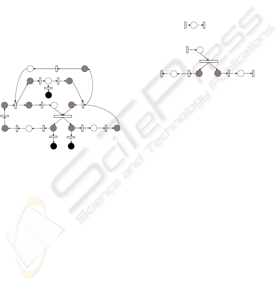
Example. Figure 1 presents an IPN model of a
system. The model has three faulty states,
represented by places p
16
, p
17
, p
18
. Function λ is
defined as λ(t
1
)=a, λ(t
3
)=b, λ(t
4
)=x, λ(t
7
)=y, λ(t
9
)=c,
λ(t
10
)=z, for others transitions λ(t
i
)=ε. Measurable
places are p
3
, p
5
, p
8
, p
12
, p
15
, P
R
= {p
4
, p
7
, p
12
}, T
R
=
{t
4
, t
7
, t
10
}, T
F
= {t
13
, t
14
, t
15
} and P
F
= {p
16
, p
17
, p
18
}.
3.2 Reduced Models
In a previous work (Arámburo-Lizárraga, et al.,
2005) we stated that the condition of event-
detectability is needed only on t
j
∈
•
P
R
and t
j
∈ P
R
•
.
This fact can be exploited in order to obtain a
reduced model containing the pertinent parts of
()
NN
MQ
0
, regarding the modelled faults in (Q,M
0
).
•
P
1
P
4
P
3
t
2
•
P
10
t
3
P
7
P
8
P
6
t
4
t
6
t
7
b
z
y
ε
ε
ε
εε
t
9
ε
•
P
2
P
5
P
9
P
11
P
12
P
13
P
14
P
15
t
1
P
16
P
17
P
18
t
5
t
8
t
10
t
11
t
12
t
13
t
14
t
15
ε
ca
ε
ε
x
Figure 1: Global model.
Definition 1. Let
()
NN
MQ
0
, be the embedded
normal behaviour included in (Q,M
0
). The reduced
model
(
)
RMRM
MQ
0
, of
(
)
NN
MQ
0
, is the subnet
induced by:
P
RM
= P
a
∪ P
b
∪ P
c
, where P
a
= {p
i
| p
i
∈ P
R
}, P
b
= {p
j
| p
j
∈ P
R••
}, and P
c
= {p
k
| p
k
∈
••
P
R
, p
k
is a
measurable place}. The sets P
b
and P
c
are
necessary only when ∃p
i
∈ P
R
, such that p
i
is
non-measurable.
T
RM
= T
in
∪ T
out
, where T
in
= {
•
p
i
| p
i
∈ P
RM
},
T
out
= {p
i
•
| p
i
∈ P
RM
}.
λ
RM
: T
RM
→Σ∪{ε},∀t
i
’
∈ T
RM
, λ(t
i
’
) = λ(t
i
), t
i
∈T
N
,
t
i
’
= t
i
.
ϕ
RM
= ϕ|
R(Q
RM
,M
0
RM
)
M
0
RM
=M
0
|
P
RM
.
The firing rules of
()
RMRM
MQ
0
,
are defined:
If t
j
∈ T
RM
is fired in (Q,M
0
) then it must be fired
in
(
)
RMRM
MQ
0
, .
If the input symbol λ(t
k
), t
k
∈ P
R•
is activated in
the system then it must be activated in
(
)
RMRM
MQ
0
, .
If ∃t
j
∈ T
RM
, s.t., t
j
is not event detectable then t
j
is fired automatically when
•
t
j
was marked.
The reduced model nodes (places and transitions)
are a copy of the original ones, and they have
associated the same input-output symbols.
Figure 2 presents the reduced model of the global
system model depicted in figure 1. Notice that in this
example the number of places is reduced and T
RM
are
only event-detectable transitions.
P
4
P
3
t
2
t
3
P
7
P
8
t
4
t
7
b
z
y
ε
ε
P
5
P
12
t
5
t
8
t
10
t
11
ε
ε
x
Figure 2: Diagnoser reduced model.
3.3 Characterisation of Diagnosability
The characterisation of input-output diagnosable
IPN is based on the partition of R(Q,M
0
) into normal
and faulty markings; all the faulty markings must be
distinguishable from other reachable markings.
Definition 2: An IPN given by (Q,M
0
) is said to
be input - output diagnosable in k < ∞ steps if any
marking M
f
∈ F is distinguishable from any other
M
k
∈ R(Q,M
0
) using any word ω ∈ Λ
k
(Q,M
f
) ∪
Λ
B
(Q,M
f
), where F = {M | ∃p
k
∈ P
F
such that
M(p
k
)>0, M ∈ R(Q,M
0
)}.
The following result extends that presented in
(Ramírez-Treviño, et al., 2007).
Theorem 1: Let (Q,M
0
) be a binary IPN, such
that
(
)
NN
MQ
0
, is live, strongly connected and event
detectable on t
j
∈
•
P
R
and t
j
∈ P
R
•
. Let {X
1
,...,X
τ
} be
the set of all T-semiflows of (Q,M
0
). If ∀
N
i
p ∈ P
N
,
(
)
•
N
i
p ∩ T
F
≠
θ
the following conditions hold:
1. ∀r, ∃j X
r
(j)≥1, where t
j
∈
(
)
•
N
i
p - T
F
,
2. ∀t
k
∈
(
)
•
N
i
p - T
F
,
•
(t
k
)={
N
i
p } and λ(t
k
) ≠ ε.
then the
IPN (Q,M
0
) is input-output diagnosable.
Proof: It is similar to that included in (Ramírez-
Treviño, et al., 2007).
DESIGN OF LOW INTERACTION DISTRIBUTED DIAGNOSERS FOR DISCRETE EVENT SYSTEMS
191
4 DISTRIBUTED DIAGNOSIS
4.1 Model Partition
In order to build a distributed diagnoser, the IPN
model (Q, M
0
) can be conveniently decomposed into
m interacting subsystems where different modules
share common nodes.
Definition 3. Let (Q,M
0
) be an IPN. The
distributed Interpreted Petri Net model
DN of
(
Q,M
0
) is a finite set of modules ℳ ={
μ
1
,
μ
2
,…,
μ
m
}
such that:
each
μ
k
∈ ℳ is an IPN subnet:
μ
k
= (N
k
,
Σ
k
,
λ
k
,
ϕ
k
),
k ∈ {1,2,…,m} modules.
•
N
k
= (P
k
, T
k
, I
k
, O
k
, M
0k
) where P
k
⊆ P, T
k
⊆ T,
I
k
(O
k
) : P
k
× T
k
→
Z
+
, s.t., I
k
(p
i
,t
j
) = I(p
i
,t
j
)
(
O
k
(p
i
,t
j
) = O(p
i
,t
j
)), ∀ p
i
∈ P
k
and ∀t
j
∈ T
k
and
M
0k
= M
0
|
Pk
•
Σ
k
= {α∈Σ⏐∃t
i
, t
i
∈T
k
, λ(t
i
) = α}
•
λ
k
: T
k
→
Σ
k
∪ {
ε
}, s.t.
λ
k
(t
i
) = λ(t
i
) and t
i
∈T
k
•
ϕ
k
: R(m
k
, M
0k
) → (Z
+
)
q
, q is restricted to the
outputs associated to
P
k
.
ϕ
k
=
ϕ
⏐
Pk
For each
μ
k
the following conditions hold:
a)
∃
μ
l
∈ℳ , s.t. T
k
∩ T
l
≠∅, P
k
∩ P
l
= {
•
t
i
∪ t
i
•
| t
i
∈
{
T
k
∩ T
l
}}, P
k
∩ P
l
are measurable places.
b)
∀p
i
∈ {P
k
– (P
k
∩ P
l
)} if p
i
∈ P
R
then p
i
••
⊂ P
k
.
c)
ICom(OCom): P
k
× T
l
→ Z
+
, s.t. I
k
(p
i
,t
j
) = I
l
(p
i
,t
j
)
(
O
k
(p
i
,t
j
) = O
l
(p
i
,t
j
)), ∀p
i
∈ P
k
and ∀t
j
∈ T
l
.
ICom and OCom represent the communication
between modules. The arcs are depicted as a
dashed line.
The obtained
DN captures the firing language
£(
Q,M
0
) in a distributed way, ∀t
x
∈ ......
kji
ttt=
σ
and
for every (
α
x
,y
x
) in ω = (α
0
,y
0
)(α
1
,y
1
)...(α
n
,y
n
) ∃
μ
k
∈ℳ
where
t
x
is fired and (α
x
,y
x
) is also generated in DN.
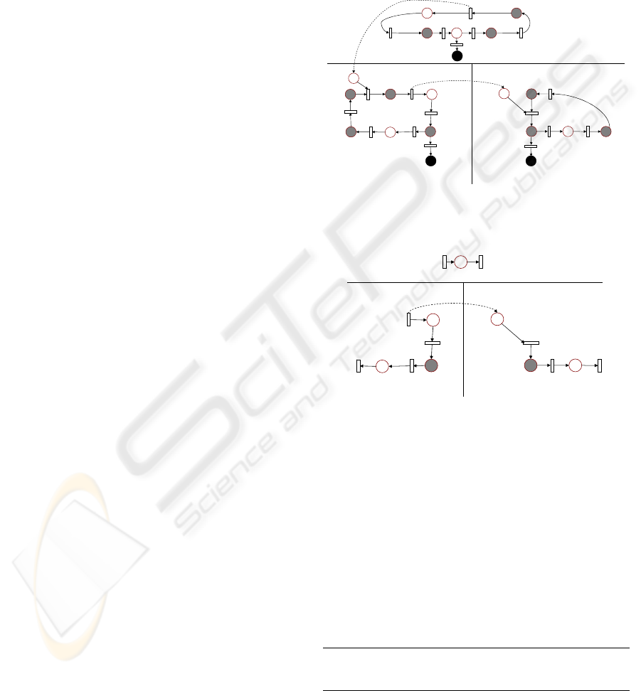
Consider the IPN system model depicted in the
Figure 1 (for the sake of simplicity, we use in the
examples the same names for duplicated nodes
(places or transitions) belonging to different
modules). Figure 3 presents the distributed
IPN, m =
3 modules,
ICom and OCom are represented by the
dashed arcs. For example we can get the sets
T
1
∩
T
2
= {t
3
} and T
1
∩ T
3
= {t
1
}, P
1
∩ P
2
= {p
3
} and P
1
∩
P
3
= {p
15
}.
We are preserving the property of event
detectability using duplicated measurable places,
which they establish the outputs that each module
needs from others modules.
4.2 Local Reduced Models
The local models can be reduced following the steps
of sub-section 3.2 and obtaining a simpler
distributed model considering the local nodes.
Definition 4. Let
μ
i
∈ℳ be an IPN module. The
local reduced model
(
)
RMRM
MQ
0
,
i
is the subnet
induced as in definition 1.
Consider the DN distributed model depicted in
figure 3, the figure 4 presents the local reduced
models where the place
p
3
is duplicated in module 2
for detecting the firing of
t
3
. The communication
between modules is represented by the dashed arcs.
•
P
1
P
4
P
3
t
2
•
P
10
t
3
P
7
P
8
P
6
t
4
t
6
t
7
b
z
y
ε
ε
ε
εε
t
9
ε
•
P
2
P
5
P
9
P
11
P
12
P
13
P
14
P
15
t
1
P
16
P
17
P
18
t
5
t
8
t
10
t
11
t
12
t
15
t
13
t
14
ε
ca
ε
ε
x
b
t
3
t
1
a
c
t
9
•
P
15
P
3
Module 3
Module 1
Module 2
Figure 3: Distributed Interpreted Petri Net.
P
4
P
3
t
2
P
7
P
8
t
4
t
7
b
z
y
ε
ε
P
5
P
12
t
5
t
8
t
10
t
11
ε
ε
x
b
t
3
P
3
Module 3
Module 1
Module 2
t
3
Figure 4: Local reduced models.
It is possible to obtain local reduced models
where the communication is eliminated, since
T
RM
n
can be event-detectable only by the local outputs.
4.3 Modular Fault Detection
The error between the system output and the local
diagnoser model output is
E
kn
=
()
k
M
ϕ
-
()
RM
kn
M
ϕ
.
The following algorithm, devoted to detect which
local faulty marking was reached in
DN, is executed
when
E
kn
≠ 0 in
μ
n
∈ℳ.
Algorithm 1. Detecting Local Faulty Markings
Inputs:
(
)
RM
kn
M
ϕ
,
RM
n
M , λ(t
i
), t
i
∈ T
RM
n
, E
kn
Outputs:
p
n
F
1.Constants:
RM
n
C
ϕ
-- local reduced normal
behaviour
2.Repeat
ICINCO 2007 - International Conference on Informatics in Control, Automation and Robotics
192

2.a. Read
()
RM
kn
M
ϕ
and λ(t
i
)
2.b. If λ(t
j
) ∈ λ(P
R
•
) then computes
δ =
(
)
RM
kn
M
ϕ
-
(
)
RM
kn
M
1−
ϕ
(a column of
RM
n
C
ϕ
)
2.c. i = index of the column of
RM
n
C
ϕ
, s.t.,
RM
n
C
ϕ
(•,i) = δ, i.e. t
i
was fired;
2.d. If
E
kn
≠ 0 then
-
∀p
n
∈ (
•
t
i
)
••
∩ P
F
n
, M
fn
(p
n
)=1
- Return (
p
n
F
)
- Sends to all modules the message “A fault
occurred in module
μ
n
in place (p
n
F
)”.
Since
()
RMRM
MQ
0
,
n
is event detectable in
•
P
R
and
P
R
•
, then step 2.b. will compute just one column
index; moreover, since
(
)
NN
MQ
0
,
n
fulfils the
conditions of theorem 1, then step 2.c. will compute
just one place.
4.4 Distributed Input-output
Diagnosability
The results of centralised diagnosability are applied
to the modules issued from the partition.
The nodes of every
μ
k
∈ℳ are partitioned into
local faulty nodes and normal nodes, i.e.,
P
k
= P
F
k
∪
P
N
k
and T
k
= T
F
k
∪ T
N
k
.
R(
μ
k
, M
0k
) denotes the reachability set of a
module
μ
k
and LF = {M
k
| ∃p
j
∈ P
F
k
, such that
M
k
(p
j
)>0, M
k
∈R(
μ
k
, M
0k
)} denotes the set of the
local faulty markings.
Λ
int
k
(
μ
k
, M
0k
) denotes the set of all input-output
sequences that lead to a marking which puts a token
into a duplicated place in other module
μ
n
, Λ
int
k
(
μ
k
,
M
0k
) = {ω| ∃σ
m
,
such that σ
m
generates ω, and
jmm
MM
m
⎯→⎯
σ
0
then M
jm
marks a p
j
s.t. p
j
∈ P
RM
m
in some module
μ
m
}.
Now, we introduce two notions for describing
degrees of diagnosability in the modules of a
distributed model.
A module is locally diagnosable if, for every
local fault we can detect it only through local
information, else it is conditionally diagnosable.
Definition 5. (Local Diagnosability) A module
μ
n
∈ℳ given by DN is said to be locally input-
output diagnosable in
k < ∞ steps if any marking M
fn
∈
LF is distinguishable from any other M
kn
∈ R(
μ
n
,
M
0n
) using any local word ω
n
∈ Λ
k
n
(
μ
n
, M
0n
) ∪
Λ
Bn
(
μ
n
, M
0n
).
Definition 6. (Conditional Diagnosability) A
module
μ
n
∈ℳ given by DN is said to be conditional
input-output diagnosable in
k < ∞ steps if any
marking
M
fn
∈ LF is distinguishable from any other
M
kn
∈ R(
μ
n
, M
0n
) using any local word ω
m
∈ Λ
k
n
(
μ
n
,
M
0n
) ∪ Λ
Bn
(
μ
n
, M
0n
) and any word ω
m
∈ Λ
int
n
(
μ
n
,
M
0n
).
Proposition 1. Let (Q,M
0
) be an IPN and DN its
corresponding distributed
IPN as stated in definition
3. If (
Q,M
0
) is input-output diagnosable as in
theorem 1 then
DN is distributed input-output
diagnosable.
Proof. Assume that (Q,M
0
) is input-output
diagnosable. There exists a finite sequence of input-
output symbols ω, s.t., ω ∈Λ
k
(Q,M
f
) ∪ Λ
B
(Q,M
f
),
and
σ = t
i
t
j
t
k
...t
m
is the firing transition sequence
whose firing generates ω s.t.
k
MM ⎯→⎯
ω
σ
0
, M
k
∈ F.
By theorem 1
M
k
is distinguishable from any other
M
k
∈ R(Q,M
0
) and (Q,M
0
) is input-output
diagnosable.
Since
DN is the distributed behaviour of (Q,M
0
),
we suppose that the sequence
σ can be fired in some
modules
μ
k
…
μ
l
,
μ
m
∈ℳ of DN, and the sequence
generates the following local markings
M
ik
∪… ∪
M
il
∪ M
im
, then M
k
= M
ik
∪… ∪ M
il
∪ M
im
, s.t. M
ik
…
M
il
∈ LN and M
im
∈ LF. Let σ
1
, σ
2
,…, σ
m
sequences s.t. σ = σ
1
σ
2
…σ
m
, suppose that σ
1
is fired
in a module
μ
k
∈ ℳ s.t.
ikk
MM
⎯
→
⎯
1
0
σ
, σ
2
is fired
in
μ
l
∈ ℳ, s.t.
ill
MM
⎯
→
⎯
2
0
σ
… , and σ
m
is fired in
μ
m
∈ ℳ, s.t.
im
m
m
MM
⎯
→
⎯
σ
0
, and σ occurs if the
sequence
σ
1
followed by a sequence σ
2
,… followed
by a sequence
σ
m
occur in the corresponding
modules. Then by definition 5 and 6
μ
m
can
distinguish any
M
im
∈ LF from any other M
km
∈
R(
μ
m
, M
0m
). Hence there exists a module
μ
m
∈ℳ
that can distinguish the corresponding faulty
marking
M
im
; as
μ
m
can be any module and
μ
m
can
be local or conditional input-output diagnosable,
therefore
DN is distributed input-output diagnosable.
Proposition 1 considers both cases (local and
conditional diagnosable modules) for establishing
the distributed input-output diagnosability of
DN.
5 REDUCING INTERACTIONS
In Section 3.2 we explained how to build reduced
models. Now, let us consider the following
assumption:
The manipulated input symbols λ(t
k
) ≠ ε are not
activated arbitrarily, only when they are enabled
at the marking
M
k
(p
k
)>0, s.t. p
k
∈
•
t
k
.
This assumption regards for building smaller
reduced models.
Definition 7. Let
(
)
NN
MQ
0
, be the embedded
normal behaviour included in (
Q,M
0
). When the
following condition holds: ∀λ(
t
k
) ≠ ε, t
k
∈ P
R•
are
fired only when it is necessary, then the reduced
model
(
)
RMRM
MQ
0
, of
(
)
NN
MQ
0
, of definition 1 is
modified considering the following sets:
P
RM
= P
a
∪ P
b
, where P
a
= {p
i
| p
i
∈ P
R
} and P
b
=
{p
j
| p
j
∈ P
R••
};
DESIGN OF LOW INTERACTION DISTRIBUTED DIAGNOSERS FOR DISCRETE EVENT SYSTEMS
193
T
RM
= T
in
∪ T
out
∪ T
af
, where T
in
= {
•
p
i
| p
i
∈
P
RM
}, T
out
= {p
i
•
| p
i
∈ P
RM
} and T
af
= {t
edx
| t
edx
∈
•
p
i
and/or t
edx
∈ p
i
•
, t
edx
is a new transition, x = 1,
2, …, z transitions non event-detectable}, T
af
is
necessary only when p
i
∈ P
RM
, such that p
i
is
non-measurable.
λ
RM
: T
RM
→Σ∪{ε},∀t
i
’
∈ {T
in
∪ T
out
}, λ(t
i
’
) = λ(t
i
),
t
i
∈T
N
, t
i
’
= t
i
. If t
i
’
∈ T
af
, t
i
’
has no input symbols.
ϕ
RM
= ϕ|
R(Q
RM
,M
0
RM
)
M
0
RM
=M
0
|
P
RM
. If ∃p
k
∈ P
RM
, s.t., M
k
(p
k
) = 0, but,
p
k
∈ t
ed
•
then M
k
(p
k
) > 0.
The firing rules of
(
)
RMRM
MQ
0
, are defined as in
definition 1 besides the following new firing rule:
The transitions that belongs to T
af
are fired
automatically, i.e,
M(
•
t
ed
) > 0 or M(t
ed
•
)= 0.
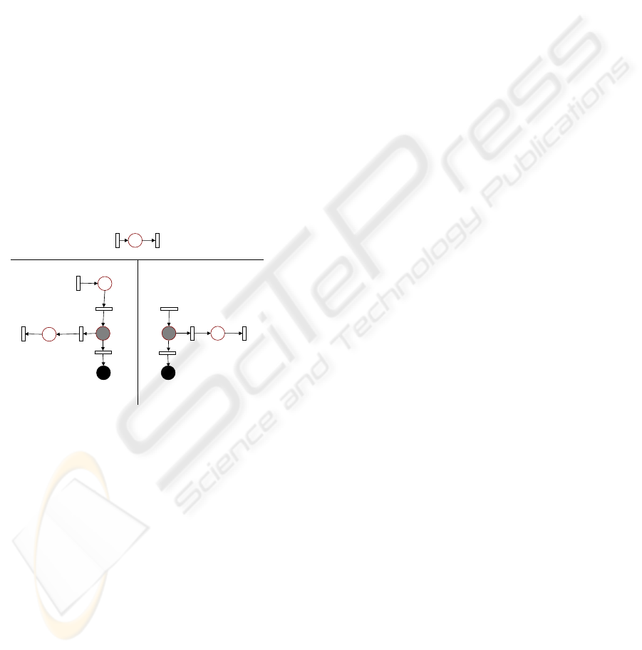
Figure 5 presents the distributed reduced model
when we consider that the input symbols are not
activated of an arbitrary way. We can see that the
transition
t
3
is not part of the reduced model of
module 2, it is replaced by a transition
t
ed1
, λ(t
ed1
) =
ε. The goal for building smaller reduced models is to
guarantee the observation of the system in critical
situations.
P
4
P
3
t
2
P
7
P
8
t
4
t
7
b
z
y
ε
εε
ε
P
5
P
12
P
16
P
17
t
5
t
8
t
10
t
11
t
13
t
14
ε
ε
x
t
ed1
t
3
Module 3
Module 1 Module 2
Figure 5: Reduced models for the centralised diagnoser.
6 CONCLUSIONS
A method for designing distributed diagnosers has
been presented. The proposed model decomposition
technique preserves the diagnosability of the global
model into the distributed one and reduces the
communication among the diagnosers. Current
research addresses reliability of distributed
diagnosers.
REFERENCES
Arámburo-Lizárraga J., E. López-Mellado, and A.
Ramírez-Treviño (2005). "Distributed Fault Diagnosis
using Petri Net Reduced Models". Proc. of the IEEE
International Conference on Systems, Man and
Cybernetics. pp. 702-707, October 2005.
Benveniste A., S. Haar, E. Fabre and C. Jara (2003).
"Distributed and Asynchronous Discrete Event
Systems Diagnosis". 42nd IEEE Conference on
Decision and Control. 2003.
Contant O, S. Lafortune and D. Teneketzis (2004).
"Diagnosis of modular discrete event systems". 7th
Int. Workshop on Discrete Event Systems Reims,
France. September, 2004.
Debouk R, S. Lafortune and D. Teneketzis (2000).
"Coordinated Decentralized Protocols for Failure
Diagnosis of Discrete Event Systems", Kluwer
Academic Publishers, Discrete Event Systems: Theory
and Applications, vol. 10, pp. 33-79, 2000.
Genc S. and S. Lafortune (2003). "Distributed Diagnosis
of Discrete-Event Systems Using Petri Nets" Proc. of
the 24th. ATPN pp. 316 - 336, June, 2003.
Genc S. and S. Lafortune (2005). “A Distributed
Algorithm for On-Line Diagnosis of Place-Bordered
Nets”. 16th IFAC World Congress, Praha, Czech
Republic, July 04-08, 2005.
Jalote P. (1994). Fault Tolerance in distributed systems.
Prentice Hall. 1994
Jiroveanu G. and R. K. Boel (2003). "A Distributed
Approach for Fault Detection and Diagnosis based on
Time Petri Nets". Proc. of CESA. Lille, France, July
2003.
Pencolé Y. "Diagnosability analysis of distributed discrete
event systems". Proc. of the 15th International
Workshop on Principles of Diagnosis. Carcassonne,
France. June 2004.
Ramírez-Treviño A., I. Rivera-Rangel and E. López-
Mellado (2003). "Observability of Discrete Event
Systems Modeled by Interpreted Petri Nets". IEEE
Transactions on Robotics and Automation, vol. 19, no.
4, pp. 557-565, August 2003.
Ramírez-Treviño, E. Ruiz Beltrán, I. Rivera-Rangel, and
E. López-Mellado (2004). A. Ramírez-Treviño, E.
Ruiz Beltrán, I. Rivera-Rangel, E. López-Mellado.
"Diagnosability of Discrete Event Systems. A Petri
Net Based Approach". Proc. of the IEEE International
Conference on Robotic and Automation. pp. 541-546,
April 2004.
Ramírez-Treviño A, E. Ruiz Beltrán, I. Rivera-Rangel, E.
López-Mellado (2007). “On-line Fault Diagnosis of
Discrete Event Systems. A Petri Net Based
Approach”. IEEE Transactions on Automation
Science and Engineering. Vo1. 4-1, pp. 31-39. January
2007.
ICINCO 2007 - International Conference on Informatics in Control, Automation and Robotics
194
