ON THE FORCE/POSTURE CONTROL OF A CONSTRAINED

SUBMARINE ROBOT

Ernesto Olgu

ın-D

ıaz and Vicente Parra-Vega

Robotics and Advanced Manufacturing, CINVESTAV-IPN, Saltillo, M

exico

Keywords:

Underwater vehicles, Force/position control, Sliding Modes Control.

Abstract:

An advanced, yet simple, controller for submarine robots is proposed to achieve simultaneously tracking of

time-varying contact force and posture, without any knowledge of its dynamic parameters. Structural proper-

ties of the submarine robot dynamic are used to design passivity-based controllers. A representative simulation

study provides additional insight into the closed-loop dynamic properties for regulation and tracking cases. A

succinct discussion about inherent properties of the open-loop and closed-loop systems ﬁnishes this work.

1 INTRODUCTION

In the last decade, we have witness a surprising leap

on scientiﬁc knowledge and technological achieve-

ments for submarine robots, from a simple torpedo

to modern UAV. Those vehicles are at the same time

tantamount scientiﬁc and technological challenges to

robotics, control and mechatronic researchers. First

efforts for free motion submarine robots were focused

for motion control, with sensing capabilities, similar

to the case of ﬁx-base robots in our labs. Of course,

stable contact for submarine robots is a more com-

plex problem in comparison to the typical force con-

trol problem of robot manipulators ﬁxed to ground be-

cause not only due complementary complex dynam-

ics such as buoyancy and added masses, but to de fact

that the vehicle reference frame is not longer inertial.

However, some tasks requires more challeng-

ing goal of establishing stable contact, which leads

us to study the problem of simultaneous force and

pose (position and orientation) control of submarine

robots. When the submarine robot achieves contact,

like pushing itself against a wall or polishing a sunken

surface vessel or manipulating tools on submarine

pipe lines, forces are presented, and little is known

about these contact forces, let alone exploit them ei-

ther for design or control. The main general reason

that this problem remains rather open is that we really

know so little about, on one hand, in how to model and

control properly a fully immersed vehicle constrained

by rigid object; and on the other hand, the submarine

force control technology lies behind system require-

ments, such as very fast sampling rates, even when

the bandwidth of the submarine robot is very low.

Despite brilliant control schemes for free motion

submarine robots in the past few years, in particular

those of (Yoerger, 1985; Smallwood, 2001; Small-

wood, 2004) those schemes does not guarantee for-

mally convergence of tracking errors, let alone si-

multaneous convergence of posture and contact force

tracking errors, there are several results that suggest

empirically that a simple PD control structure be-

haves as stiffness control for submarine robots. So far

the simultaneous convergence of time-varying contact

forces and posture remains an open problem for the

PD-like controller (notice that for submarine robots

the role of model-free controllers are very important

because it is very hard to known exactly the dynamic

model and its dynamic parameters).

Recently, some efforts have focused on how to

obtain simple control structures to control the time-

varying pose of the UAV under the assumption that

the relative velocities are low. For force control, vir-

tually none complete control system has been pub-

lished. However, to move forward more complex

force controllers, we believe that more understanding

of the structural properties of submarine robots in sta-

ble contact to rigid objects are required.

Olguín-Díaz E. and Parra-Vega V. (2007).

ON THE FORCE/POSTURE CONTROL OF A CONSTRAINED SUBMARINE ROBOT.

In Proceedings of the Fourth International Conference on Informatics in Control, Automation and Robotics, pages 19-28

DOI: 10.5220/0001631800190028

 SciTePress

To understand more about this problem, we show

that the open-loop rigid dynamics of submarine robots

subject to holonomic constraints (rigid contact) ex-

hibits similar properties of ﬁxed-base robots. Then

almost any force/position control scheme with the

proper adequation can be used. In this paper we

have chosen the orthogonalization principle (Parra-

Vega and Arimoto, 1996) to propose a simple con-

troller with advanced tracking stability properties.

1.1 Contribution

Despite the complexity of the problem, in this pa-

per, the performance of a robot submarine carry-

ing out a very simple contact tasks under a novel

orthogonalization-based model-free controller is an-

alyzed and discussed, with emphasize on structural

properties. The closed-loop shows robust tracking of

time-varying contact force and posture, without any

knowledge of submarine dynamics. The proposed

controller stands itself as a new controller which guar-

antees simultaneous tracking of submarine robot with

a model-free decentralized control structure.

1.2 Organization

Section 2 introduces the nonlinear differential alge-

braic equations of the robot submarine dynamics in

error coordinates. Section 3 presents the control de-

sign. Simulation data is presented for a Testbed robot

of IFREMER in 4, and ﬁnally section 5 discusses

some structural properties useful for further under-

stand robot submarine in contact tasks. Conclusions

are stated in Section 6.

2 THE MODEL

2.1 A Free Floating Submarine

The model of a submarine can be obtained via Kirch-

hoff formulation (Fossen, 1994), the inclusion of hy-

drodynamic effects such as added mass, friction and

buoyancy and the account of external forces/torques

like contact effects (Olgu

ın-D

ıaz, 1999). The model

is then expressed by the next set of equations:

ν+C

(ν)ν+ D

(·)ν+ g

(q) = u+ F

(v)

(1)

ν = J

(q)˙q (2)

From this set, (1) is called the dynamic equation while

(2) is called the kinematic equation. Both had been

used long widely to express the dynamical behavior

of free moving object in the 3D space.

The generalized coordinates vector q ∈ IR

given on one hand by the 3 Cartesian positions x, y,z

of the origin of the submarine frame (Σ

) with respect

to a inertial frame (Σ

) ﬁxed in some place on the sur-

face of the Earth; and on the other hand by any set of

attitude parameters that represent the rotation of the

vehicle’s frame with respect to the inertial one. Most

common sets of attitude representation such a Euler

angles, in particular roll-pitch-yaw (φ, θ,ψ), use only

3 variables (which is the minimal number of orien-

tation variables). Then, for a submarine vehicle, the

generalized coordinates q = (x

,φ

,θ

,ψ

) rep-

resents its 6 degrees of freedom.

The vehicle’s velocity ν ∈ IR

is the vector repre-

senting both linear and angular velocity of the subma-

rine expressed in its own vehicle’s frame. This vector

is then deﬁned as ν = (v

(v)

,ω

(v)

)

. The relation-

ship between this vector and the generalized coordi-

nates is given by the kinematic equation. The linear

operator J

(q) ∈ IR

6×6

in (2) is built by the concate-

nation of two transformations. The ﬁrst is deﬁned as:

(q) =



I 0

0 J

(φ

,θ

,ψ

)



∈ IR

6×6

Where J

∈ IR

3×3

is an operator that converts

time derivatives of attitude (orientation) parameters

in angular velocity: ω

(0)

= J

(θ

)

, with θ

(φ

,θ

,ψ

)

deﬁned as the orientation parameter vec-

tor. The operator J

(q) maps the ﬁrst time derivative

of the generalized coordinates to linear and angular

velocities of the submarine vehicle, both expressed in

the inertial frame Σ

The second operator transforms a 6 dimension

tensor from the inertial frame to vehicle’s frame by

(q) = diag{R

} ∈ IR

6×6

. Thus the Jacobian of

the vehicle used in the kinematic equation is a linear

operator deﬁned as:

(q) = J

(q)J

(q)

In the dynamic equation (1), matrices

(ν),D

(·) ∈ IR

6×6

are respectively Inertia

matrix, Coriolis matrix and Damping matrix. M

includes the terms of classical inertia plus the hydro-

dynamic coefﬁcients of the added mass effect (due

to the amount of extra energy needed to displace the

surrounding water when the submarine is moving).

This Inertia matrix is constant, deﬁnite positive and

symmetric only when the submarine is complete

immersed and the relative water incidence velocity is

small (Fossen, 1994). This condition is met for most

common activities of a ROV, for example during

sampling recollection in not shallow waters. The

Coriolis vector C

(ν)ν represents the Coriolis forces,

gyroscopic terms of the classical inertia effects plus

ICINCO 2007 - International Conference on Informatics in Control, Automation and Robotics

the quadratic velocity terms induced by the added

mass. The Coriolis matrix in this representation

does not depend on the position but only on the

velocity, in contrast to the same expression for a

Robot Manipulator (Spong M.W., 1989). However

it fulﬁlls the classic relationship for Lagrangian

systems:

− 2C

(ν) = Q; Q + Q

= 0, and is

indeed skew symmetric. The Damping matrix

represents all the hydrodynamic effects of energy

dissipation. For that reason it is a strictly positive

deﬁnite matrix, D

(q,ν,t) > 0 (Fossen, 1994). Its

arguments are commonly the vehicle’s orientation

,θ

,ψ

, the generalized velocity ν, and the velocity

of the surrounding water. The diagonal components

represents the drag forces while the off-diagonal

components represent the lift forces.

Finally, vectors g

(q),u,F

(v)

∈ IR

are all force

wrenches (force-torque vector) in the vehicle’s frame.

They represent respectively: gravity, input control

and the contact force. Gravity vector includes buoy-

ancy effects and it does not depend on velocity but

on the orientation (attitude) of the submarine with re-

spect to the inertial frame. The contact force wrench

is the one applied by the environment to the subma-

rine. The input control are the forces/torques induced

by the submarine thrusters in the vehicle frame.

The dynamic model (1)-(2) can be rearranged by

replacing (2) and its time derivative into (1). The re-

sult is one single equation model:

(q)¨q+C

(q, ˙q)˙q+ D

(·)˙q+ g

(q) = u

+ τ

(3)

which has the form of any Lagrangian system. Its

components fulﬁlls all properties of such systems i.e.

deﬁnite positiveness of inertia and damping matrices,

skew symmetry of Coriolis matrix and appropriate

bound of all components (Sagatun, 1991).

The control input in this equation is obtained by a

linear transformation of the real input using the linear

operator given by the kinematic equation:

= J

(q)u. (4)

This last equation becomes important because it re-

lates the nominal control signal u

to be designed in

the general coordinates space with the real physical

input u that shall be implemented in the real vessel.

The contact effect is also obtained by the same trans-

formation. However it can be expressed directly from

the contact wrench in the inertial frame (Σ

) by the

next relationship

= J

(q)F

(v)

= J

(q)F

(0)

(5)

where the contact force F

(0)

is the one expressed in

the inertial frame. By simplicity it will be noted

as F

from this point further. The relationship with

the one expressed in the vehicle’s frame is given by

= J

(q)F

(v)

. This wrench represents the contact

forces/torques exerted by the environment to the sub-

marine as if measured in a non moving (inrtial) frame.

These forces/torques are given by the normal force of

an holonomic constraint when in contact and the fric-

tion due to the same contact. For simplicity in this

work, tangential friction is not considered.

2.2 Contact Force Due to a Holonomic

Constraint

A holonomic constraint can be expressed as a function

of the generalized coordinates of the submarine as

ϕ(q) = 0 (6)

with ϕ(q) ∈ IR

. The number r stand for the num-

ber of contact points between the submarine and the

motionless rigid object. Stable contact appears only

when the robot submarine does not deattach from the

object modeled by ϕ(q) = 0. In this case, the time

derivatives of this constraint are zero

ϕ(q)

= 0; ∀ n ≥ 1 (7)

For n = 1 the last constraint becomes:

ϕ(q) = J

(q)˙q = 0 (8)

where J

(q) =

∂ϕ(q)

∂q

∈ IR

r×n

is the constraint jaco-

bian. Last equation means that velocities of the sub-

marine in the directions of constraint jacobian are re-

stricted to be zero. This directions are then normal to

the constraint surface ϕ(q) at the contact point. As

a consequence, the normal component of the contact

force has exactly the same direction as those deﬁned

by J

(q). Then the contact force wrench can be ex-

pressed as

= J

ϕ+

(q)λ (9)

where J

ϕ+

(q)

△

is a normalized version of the

constraint jacobian; and λ is the magnitude of the

normal contact force at the origin of vehicle frame:

λ = kF

The free moving model expressed by (1)-(2),

when in contact with the holonomic constraint can be

rewritten as:

ν+ h

(q,ν,t) = u+ J

(q)J

ϕ+

(q)λ (10)

ν = J

(q)˙q (11)

ϕ(q) = 0 (12)

where h

(q,ν,t) = C

(ν)ν+ D

(q,ν,t)ν + g

(q).

ON THE FORCE/POSTURE CONTROL OF A CONSTRAINED SUBMARINE ROBOT

Equivalently, the model (3) is also expressed as

(q)¨q+ h

(q, ˙q,t) = u

+ J

(q)λ (13)

ϕ(q) = 0 (14)

with h

(q, ˙q,t) = C

(q, ˙q)˙q+ D

(q, ˙q,t)˙q+ g

(q) and

(q) = J

ϕ+

(q)J

(q). Equations (13)-(14) are a set

of Differential Algebraic Equations index 2 (DAE-2).

To solve them numerically, a DAE solver is required.

This last representation has the same structure and

properties as those reported in (Parra-Vega, 2001).

2.3 Numerical Considerations

To compute the value of λ, the constrained La-

grangian that fulﬁls the constrained movement, can be

calculated using the second derivative of (7):

ϕ(q) =

0. Then using the dynamic equation (either of them)

and after some algebra its expression becomes either:

λ =

−1

ϕ+

−1



−1



− u



−



−1





(15)

−1



−1

− u

) −

˙q



(16)

The set of equations (10)-(11)-(15) or the set (13)-

(16) describes the constrained motion of the subma-

rine when in contact to inﬁnitely rigid surface de-

scribed by (6). Numerical solutions of these sets can

be obtained by simulation, however the numerical so-

lution, using a DAE solver, can take too much effort

to converge due to the fact that these sets of equa-

tion represent a highly stiff system. In order to min-

imize this numerical drawback, the holonomic con-

straint has been treated as a numerically compliant

surface which dynamic is represented by

ϕ(q) + D

ϕ(q) + Pϕ(q) = 0 (17)

This is known in the force control literature of robot

manipulators as constrained stabilization method,

which bounds the nonlinear numerical error of in-

tegration of the backward integration differentiation

formula. With a appropriate choice of parameters

P ≫ 1 and D ≫ 1, the solution of ϕ(q,t) → 0 is

bounded. This dynamic is chosen to be fast enough to

allow the numerical method to work properly. In this

way, it is allowed very small deviation on the com-

putation of λ, typically in the order of −10

or less,

which may produce, according to some experimental

comparison, less than 0.001% numerical error. Then,

the value of the normal contact force magnitude be-

comes:

λ =

−1

ϕ+

−1



−1



− u



−



−1



ν− DJ

−1

ν− Pϕ(q)



(18)

−1



−1

− u

) −

˙q

−DJ

˙q− Pϕ(q)



(19)

It can be pointed out that equation (19) compute the

contact force magnitude using the generalized coor-

dinates variables only. From this equation, desired

force can be easily obtained. Also note that the pre-

liminary inverse operator is only expressed by the in-

ertia matrix inverse and the two constraint jacobians.

The ﬁrst is the gradient of the contact surface, while

the second is the normalized gradient with a simple

kinematic variation given by the operator J

3 CONTROL DESIGN

The introduction of a so called Orthogonalization

Principle has been a key in solving, in a wide sense,

the force control problem of a robot manipulators.

This physical-based principle states that the projec-

tion (dot product) of contact forces and joint gener-

alized velocities is zero. Then passivity arises from

torque input to generalized velocities. To preserve

passivity, then, the closed-loop system must satisfy

the passivity inequality for controlled generalized er-

ror velocities. This is true for robot manipulators with

ﬁxed frame, and here we prove that this also hap-

pens with robot whose reference frame is not inertial

(ﬁxed).

3.1 Orthogonalization Principle and

Linear Parametrization

Similar to (Liu et al., 1997), an orthogonal projection

of J

(q) arises onto the tangent space at the contact

point. This tangent space can be calculated by the

deﬁnition of the following operator

Q(q)

△

= I

− J

(q)J

(q) ∈ IR

n×n

(20)

where I

is an identity matrix of proper size. No-

tice that rank{Q(q)} = n− r since rank{J

(q)} = r.

Also notice that Q˙q = ˙q due to the deﬁnition of Q and

(8). Therefore, and according to the Orthogonaliza-

tion Principle the integral of (τ, ˙q) is upper bounded

by −

H (t

), for H (t) = K + P, and passivity arise

ICINCO 2007 - International Conference on Informatics in Control, Automation and Robotics

for fully immersed submarines without inertial frame.

Therefore, passivity-based control is a powerful op-

tion to control such systems.

On the other hand it is known that equation (13)

can be linearly parameterized as follows

(q)¨q+C

(q, ˙q)˙q+ D

(·)˙q+ g

(q) = Y(q, ˙q, ¨q)Θ

(21)

where the regressor Y(q, ˙q, ¨q) ∈ IR

n×p

is composed

of known nonlinear functions and Θ ∈ IR

by p un-

known but constant parameters.

3.2 Change of Coordinates

A variation Y

of regressor Y can be designed such

that

(q, ˙q, ˙q

, ¨q

)Θ = (22)

(q)¨q

+ [C

(q, ˙q) + D

(·)] ˙q

+ g

(q)

where ( ˙q

, ¨q

) are some time functions yet to be de-

ﬁned. Then the open loop equation (13) can be written

by adding and subtracting (22) as

(q)˙s = −[C

(q, ˙q) + D

(·)]s (23)

−Y

(q, ˙q, ˙q

, ¨q

)Θ+ J

(q)λ+ u

where s

△

= ˙q − ˙q

is called the extended error. The

problem of control design for the open loop equation

(23) is to ﬁnd u

such that exponential convergence

arises when Y

Θ is not available.

3.3 Orthogonal Nominal Reference

Consider that q

(t) and λ

(t) are the desired trajecto-

ries functions for position and contact force. Consider

as well, the tracking errors deﬁned as ˜q

△

= q(t) − q

(t)

for position error while

△

= λ(t) − λ

(t) stand for the

force contact error. Consider also the next set of deﬁ-

nitions:

△

˜q+ σ˜q (24)

△

= S

−α(t−t

)

(25)

△

= S

− S

(26)

△

λdt (27)

△

= S

−η(t−t0)

(28)

△

= S

− S

(29)

with α > 0, η > 0. Finally, consider the following

reference ˙q

function:

˙q

= Q



˙q

− σ˜q+ S

− γ

sgn{S

(t)}dt



(30)

+βJ



− S

+ γ

sgn{S

(t)}dt



where the parameters β, σ, γ

and γ

are constant ma-

trices of appropriate dimensions; and sgn(y) stands

for the entrywise signum function of vector y,

Using (30) into s, it arises

s = Q(q)S

− βJ

(q)S

(31)

where the orthogonal extended position and force

manifolds S

and S

, respectively, are given by

= S

+ γ

sgn(S

(ς))dς (32)

= S

+ γ

sgn(S

(ς))dς (33)

Notice that although the time derivative of ˙q

discontinuous, it will not be used in the controller.

In the next subsection we show that if

are

bounded, and for large enough γ

,γ

, then simultane-

ous tracking of contact force and posture is achieve.

3.4 Model-Free Second Order Sliding

Mode Control

Consider the following nominal continuous control

law:

= −K



Q(q)s

− βJ

(q)s



(34)

(q)



−λ

+ S



+γ

(q)



tanh(µS

) + η

sgn(S

)



with µ > 0 and K

= K

> 0,∈ IR

n×n

. This nominal

control, designed in the q-space can be mapped to the

original coordinates model, expressed by the set (1)-

(2), using the next relationship

u = J

−T

(q)u

(35)

thus, the physical controller u is implemented in terms

of a key inverse mapping J

−T

3.4.1 Closed-loop System

The open loop system (23) under the continuous

model-free second order sliding mode control (34)

yields to

˙s = −[C

+ D

+ K

]s−Y

Θ (36)



λ+ ηS



+ γ

Z + τ

∗

+γ



sgn(S

) + η

sgn(S

)



ON THE FORCE/POSTURE CONTROL OF A CONSTRAINED SUBMARINE ROBOT

where Z = tanh(µS

) − sgn(S

) and τ

∗

≡ 0 is the

virtual control input for the passivity analysis.

3.4.2 Stability Analysis

Theorem 1 Consider a constrained submarine (13)-

(16) under the continuous model-free second order

sliding mode control (34). The Underwater system

yields a second order sliding mode regime with local

exponential convergence for the position, and force

tracking errors.

Proof. A passivity analysis hS, τ

∗

i indicates that

the following candidate Lyapunov function V quali-

ﬁes as a Lyapunov function

V =

s+ βS

) (37)

for a scalar β > 0. The time derivative of the Lya-

punov candidate equation immediately leads to

V = −s

+ D

)s− βηS

− s

Z (38)

≤ −s

s− βηS

+ kskkY

Θk

+kskkγ

kkJ

kkZk

≤ −s

s− βηS

+ kskkεk

where it has been used the skew symmetric property

M − 2C(q, ˙q), the boundedness of both the feed-

back gains and submarine dynamic equation (there

exists upper bounds for M,C(q, ˙q),g(q), ˙q

, ¨q

), the

smoothness of ϕ(q) (so there exists upper bounds for

and Q(q)), and ﬁnally the boundedness of Z. All

these arguments establish the existence of the func-

tional ε. Then, if K

, β and η are large enough such

that s converges into a neighborhood deﬁned by ε cen-

tered in the equilibrium s = 0, namely

s → ε as t → ∞ (39)

This result stands for local stability of s provided that

the state is near the desired trajectories for any initial

condition. This boundedness in the

∞

sense, leads to

the existence of the constants ε

> 0 and ε

> 0 such

that

| < ε

, (40)

| < ε

(41)

An sketch of the local convergence of S

is as fol-

lows

. Locally, in the n − r dimensional image of Q,

we have that S

∗

= QS

∈ IR

. Consider now that un-

der an abuse of notation that S

= S

∗

, such that for

The strict analysis follows Liu, et. al.

small initial conditions, if we multiply the derivative

of S

in (32) by S

, we obtain

= −γ

| + S

(42)

≤ −γ

| + |S

Substituting (40) into (42) yields

≤ −(γ

− ε

)|S

| (43)

where γ

must be chosen such that γ

> ε

. The equa-

tion (43) is precisely the condition for the existence of

a sliding mode at S

(t) = 0. The sliding mode is es-

tablished in a time t ≤ |S

)|/(γ

−ε

), and accord-

ing to the deﬁnition of S

(below (32)), S

) = 0,

which simply means that S

(t) = 0 for all time. We

see that if we multiply the derivative of (33) by S

we obtain

= −γ

| + S

(44)

≤ −γ

| + |S

substituting (41) into (44) yields

≤ −(γ

− ε

)|S

| (45)

where γ

must be chosen such that γ

> ε

. The equa-

tion (45) is precisely the condition for the existence

of a sliding mode at S

(t) = 0. The sliding mode

is established in a time t ≤ |S

)|/(γ

− ε

) and,

according to (33), S

) = 0, which simply means

that S

(t) = 0 for all time, which simply implies that

λ → λ

exponentially fast.

4 SIMULATION RESULTS

Force control of submarine robots is in its infancy,

therefore simulations study must be kept rather simple

to enter into the intricacies of the numerical solutions.

Later on, the complexity of the simulation study will

be be increased such that underwater disturbances can

include unmodelled submarine dynamics, such as lat-

eral marine current with high Reynolds number, to

mention one. Then, the simulation study has been

made on a simpliﬁed platform of a real submarine.

Data has been obtained from the Vortex system of

IFREMER (IFREMER, 1992). Simulator presents

only vertical planar results (only in the x-z plane), so

the generalized coordinates for this case of study are:

q =









(46)

The vehicle velocities are

v =









(47)

ICINCO 2007 - International Conference on Informatics in Control, Automation and Robotics

where u

and w

are linear velocities (surge and

heave) and q

is the angular velocity in the x-z plane.

The holonomic constraint is given by a vertical sur-

face located at 2 meters from the origin. This is ex-

pressed as:

ϕ(q) ≡ x− 2 (48)

Initial conditions were calculated to be at the con-

tact surface with no force. Simulations with simple

PD were also performed as a comparison tool. The

model-free control parameters are as follows:

α β γ

4 0.025 0.0025 10

−3

σ η µ

200

5 1000 1

where

is made by the diagonal values of the con-

stant Inertia matrix when expressed in the vehicle’s

frame. For de PD the gains were deﬁned as K

100

and K

= 20

. The numerical dynamic in-

duced in the constraint surface were performed with

P = 9x10

and D = 36x10

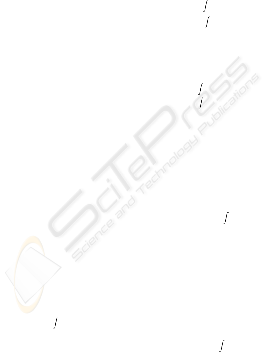
4.1 Set-Point Control Case

The task is very simple. It consist on a change of deep,

from 1m to 1.5m, and orientation from 5 degrees to 0,

while the submarine remains in contact with a con-

stant contact force of 170N.

0 0.5 1 1.5 2

1.99

1.995

2.005

2.01

x position [m]

0 0.5 1 1.5 2

−1

−0.5

0.5

Surge (u

) [m/s]

0 0.5 1 1.5 2

1.2

1.4

1.6

Deep [m]

0 0.5 1 1.5 2

0.5

1.5

Heave (w

) [m/s]

0 0.5 1 1.5 2

time [sec]

Orientation [deg]

0 0.5 1 1.5 2

−0.4

−0.3

−0.2

−0.1

0.1

time [sec]

Angular velocity [rad/s]

Figure 1: Generalized coordinates q and vehicle velocities

ν, in vehicle’s frame (continuous line for model-free second

order sliding mode control, dotted line for PD control).

Figures 1 and 2 shows respectively position, ve-

locity and force inputs. The difference in settling time

has been explicitly computed in order to visualize the

qualitative differences. In any case, this time inter-

val can be modiﬁed with appropriate tuning of gain

parameters. Notice that there is some transient and

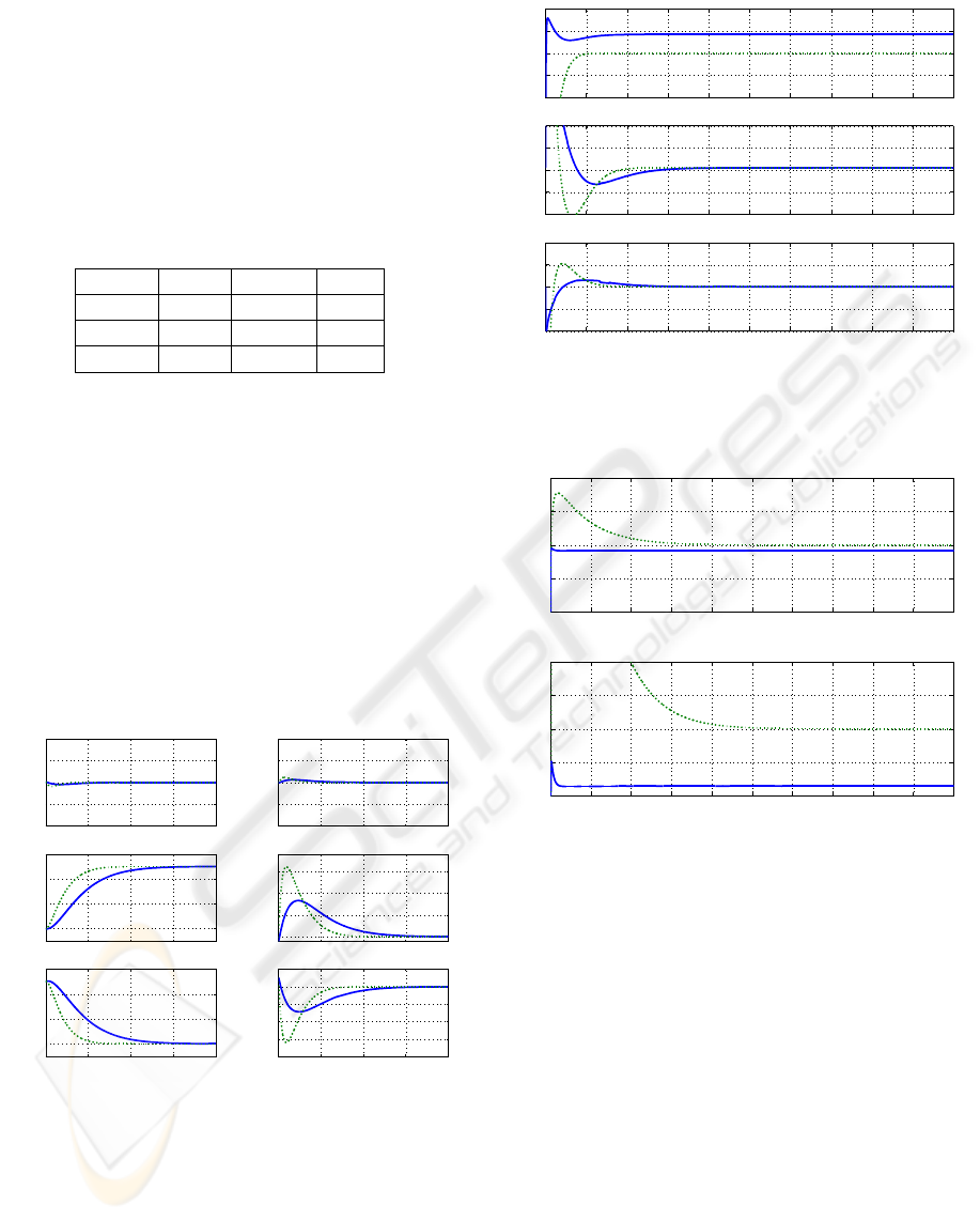
0 0.5 1 1.5 2 2.5 3 3.5 4 4.5 5

−400

−200

200

400

Input force on x [N]

0 0.5 1 1.5 2 2.5 3 3.5 4 4.5 5

−400

−200

200

400

Input force on z [N]

0 0.5 1 1.5 2 2.5 3 3.5 4 4.5 5

−40

−20

time [sec]

Input torque [Nm]

Figure 2: Inputs controlled forces u, in vehicle’s frame (con-

tinuous line for model-free second order sliding mode con-

trol, dotted line for PD control).

0 0.1 0.2 0.3 0.4 0.5 0.6 0.7 0.8 0.9 1

−2000

−1000

1000

2000

Contact force [N]

0 0.1 0.2 0.3 0.4 0.5 0.6 0.7 0.8 0.9 1

−200

−100

100

200

time [sec]

Contact force (detail) [N]

Figure 3: Contact force magnitude λ (continuous line for

model-free second order sliding mode control, dotted line

for PD control).

variability in the position of the contact point in the

the direction normal to that force (the x coordinate).

This is more visible in the velocity curve where veloc-

ity in the x direction should not occur if the constraint

is inﬁnitely rigid. The same transients are present in

the force graphic where a noticeable difference be-

tween simple PD and model-free second order sliding

mode control is present. The big difference is that al-

though PD can regulate with some practical relative

accuracy it is not capable to control force references,

either constant nor variable. Figure 3 shows the tran-

sient of the contact force magnitude λ (only the 1st

second is shown). The second window shows with

more detail the transient in this contact force due to

the numerical modiﬁcation. In this graphic is is clear

that no force is induced with the PD scheme. In the

ON THE FORCE/POSTURE CONTROL OF A CONSTRAINED SUBMARINE ROBOT

0 0.5 1 1.5 2

−10

−8

−6

−4

−2

x 10

−4

x error [m]

0 0.5 1 1.5 2

−400

−200

200

400

Force contac error [N]

0 0.5 1 1.5 2

−0.5

−0.4

−0.3

−0.2

−0.1

0.1

time [sec]

Deep error [m]

0 0.5 1 1.5 2

−1

time [sec]

Orientation error [deg]

Figure 4: Set-point control errors: ˜q = q(t) − q

and

λ =

λ(t)− λ

(continuous line for model-free second order slid-

ing mode control, dotted line for PD control).

0 1 2 3 4 5

−0.1

−0.05

0.05

0.1

0.15

0 0.5 1 1.5 2

−0.01

−0.005

0.005

0.01

0 1 2 3 4 5

−0.4

−0.3

−0.2

−0.1

0.1

0.2

0.3

time [sec]

0 0.5 1 1.5 2

−0.04

−0.02

0.02

0.04

time [sec]

Figure 5: Control variables S

and S

for the model-free

second order sliding mode control.

case of the model-free 2nd order sliding mode, force

set-point control is achieved very fast indeed. Fig-

ure 4 shows the set-point control error for position (3

curves) and force. Is again evident the substantial dif-

ference in schemes for force control. Figure 5 shows

the convergence of the extended position and force

manifolds. They do converge to zero and induce there

after the sliding mode dynamics.

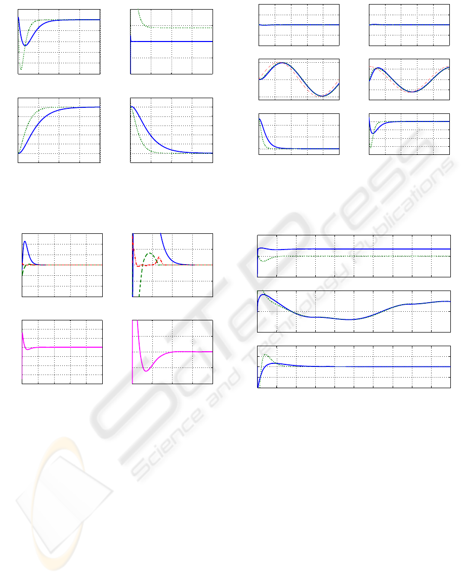
4.2 Tracking Control Case

This task differs from the set-point control case in that

the deep is a periodic desired trajectory center at 1

meter deep with 1 meter amplitude (pick to pick) and

a 5 sec period. Contact desired force remains constant

at 170N.

0 1 2 3 4 5

1.99

1.995

2.005

2.01

x position [m]

0 1 2 3 4 5

−1

−0.5

0.5

Surge [m/s]

0 1 2 3 4 5

0.5

1.5

Deep [m]

0 1 2 3 4 5

−1

−0.5

0.5

Heave [m/s]

0 1 2 3 4 5

time [sec]

Orientation [deg]

0 1 2 3 4 5

−0.4

−0.3

−0.2

−0.1

0.1

time [sec]

Angular velocity [rad/s]

Figure 6: Generalized coordinates q and vehicle velocities

ν, in vehicle’s frame for the tracking case (continuous line

for model-free second order sliding mode control, dotted

line for PD control, dashed line for the tracking reference).

0 0.5 1 1.5 2 2.5 3 3.5 4 4.5 5

−500

500

Input force on x [N]

0 0.5 1 1.5 2 2.5 3 3.5 4 4.5 5

−500

500

Input force on z [N]

0 0.5 1 1.5 2 2.5 3 3.5 4 4.5 5

−40

−20

time [sec]

Input torque [Nm]

Figure 7: Inputs controlled forces u, in vehicle’s frame (con-

tinuous line for model-free second order sliding mode con-

trol, dotted line for PD control).

As for the set-point control case, the position error

and velocities in the constrained direction remain very

small as can be see in ﬁgure 6. Also in this ﬁgure, the

deep response has a lag from the tracking reference.

As for the input control forces u the steady state re-

semble to those of the set-point control. For the deep

coordinate, the control input tends to to be the same

after some relative small time. Again, the PD does

not provide any force in the constraint direction. The

last can be veriﬁed in ﬁgure 8 where, for the PD case,

there is no contact force although the position of the

contact point is indeed in contact. For the model-free

2nd order sliding mode control, the contact force has

the same shape as for the set-point control case. The

same transient, due to the numerical consideration for

ICINCO 2007 - International Conference on Informatics in Control, Automation and Robotics

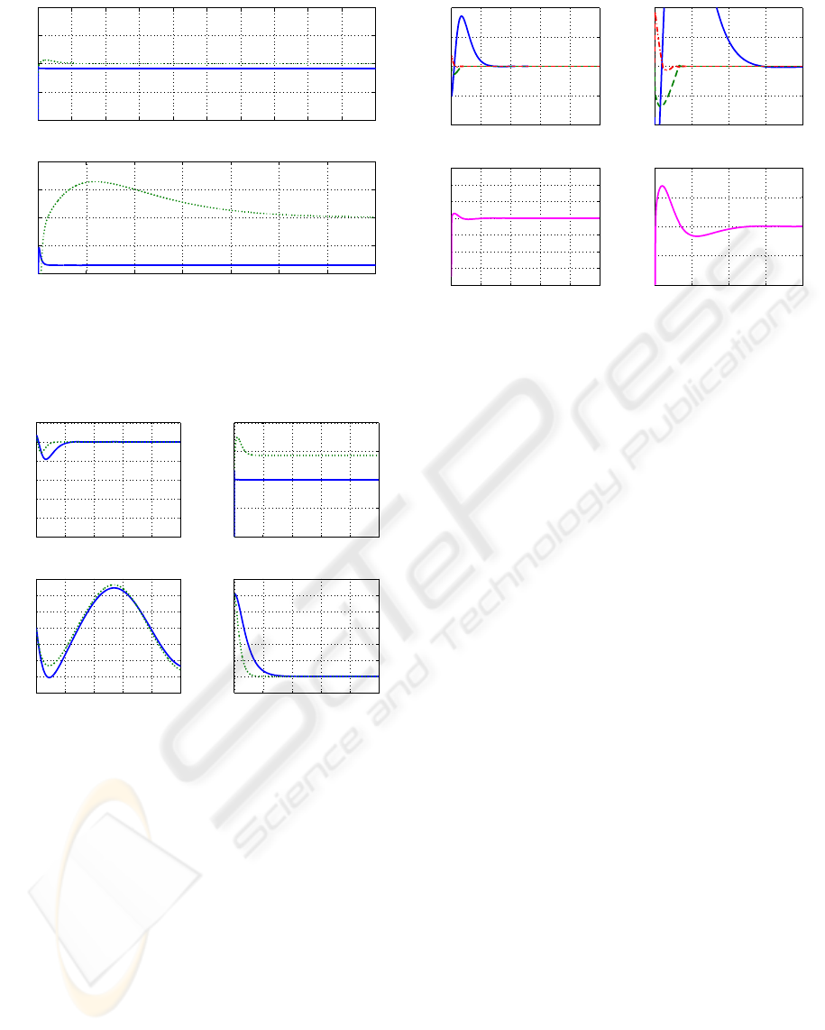
0 0.5 1 1.5 2 2.5 3 3.5 4 4.5 5

−2000

−1000

1000

2000

time [sec]

Contac force [N]

0 0.1 0.2 0.3 0.4 0.5 0.6 0.7

−200

−100

100

200

time [sec]

Contac force (detail) [N]

Figure 8: Contact force magnitude λ (continuous line for

model-free second order sliding mode control, dotted line

for PD control).

0 1 2 3 4 5

−10

−8

−6

−4

−2

x 10

−4

x error [m]

0 1 2 3 4 5

−400

−200

200

400

Force contact error [N]

0 1 2 3 4 5

−0.2

−0.15

−0.1

−0.05

0.05

0.1

0.15

time [sec]

Deep error [m]

0 1 2 3 4 5

−1

time [sec]

Orientation error [deg]

Figure 9: Set-point control errors: ˜q = q(t) − q

and

λ =

λ(t)− λ

(continuous line for model-free second order slid-

ing mode control, dotted line for PD control).

the almost rigid constraint surface, is present. The

tracking errors for the x position and force has been

reduced for the PD case certainly due to numerical

initial conditions. In the tracking of deep, the model-

free 2nd order sliding mode has apparently the same

performance as the simpler PD controller. As it has

been pointed out by other authors, for this kind of sys-

tem, the PD controller remains as the best and simpler

controller for position tracking. However, it does not

track any force reference, which is the essence of the

model-free 2nd order sliding mode control. The last

ﬁgure 10 shows the convergence of the extended posi-

tion and force manifolds to zero and induce there after

the sliding mode dynamics.

0 1 2 3 4 5

−0.05

−0.025

0.025

0.05

0 0.5 1 1.5 2

−0.01

−0.005

0.005

0.01

0 1 2 3 4 5

−0.4

−0.3

−0.2

−0.1

0.1

0.2

0.3

0 0.5 1 1.5 2

−0.04

−0.02

0.02

0.04

Figure 10: Control variables S

and S

for the model-free

second order sliding mode control.

5 SOME DISCUSSIONS ON

STRUCTURAL PROPERTIES

In the beginning of this study, we were expecting an

involved control structure for submarine robots, in

comparison to ﬁxed-base robots, with additional con-

trol terms to compensate for hydrodynamic and buoy-

ancy forces. However, surprisingly, no additional

terms were required! Due to judicious treatment of

the mathematical model, and careful mapping of ve-

locities through jacobians in vehicle frame and gen-

eralized frame, it sufﬁces only proper mapping of the

gradient of contact forces. This results open the door

to study similar force control structures developed for

ﬁxed-base robots, and so far, the constrained subma-

rine robot control problem seems now at reach.

5.1 Properties of the Dynamics

As it as pointed out in Section 2, the model of a sub-

marine robot can be expressed in either a self space

(where the inertia matrix is constant for some con-

ditions that in practice are not difﬁcult to met) or

in a generalized coordinate space (in which the in-

ertial matrix is no longer constant but the model is

expressed by only one equation, likewise the kine-

matic lagrangian chains). Both representations has

all known properties of lagrangian systems such skew

symmetry for the Coriolis/Inertia matrix, bound-

less of all the components, including buoyancy, and

passivity preserved properties for the hydrodynamic

added effects. The equivalences of these representa-

tion of the same model can be found by means of the

kinematic equation. The last one is a linear opera-

tor that maps generalized coordinates time derivative

ON THE FORCE/POSTURE CONTROL OF A CONSTRAINED SUBMARINE ROBOT

with a generalized physical velocity. This relationship

is specially important for the angular velocity of a free

moving object due to the fact that time derivative of

angular representations (such a roll-pitch-yaw) do not

stand for the angular velocity. However, there is al-

ways a correspondence between these vectors. For

external forces this mapping is indeed important. It

relates a physical force/torque wrench to the general-

ized coordinates q = (x

,φ

,θ

,ψ

) whose last

3 components does not represent a unique physical

space. In this work, such mapping is given by J

and

appears in the contact force mapping by the normal-

ized operator J

. The operator J

can be seen as the

difference of a Analytical Jacobian and the Geometric

Jacobian of a robot manipulator.

5.2 The Controller

Notice that the controller exhibits a PD structure

plus a nonlinear I-tame control action, with nonlin-

ear time-varying feedback gains for each orthogonal

subspace. It is in fact a decentralized PID-like, coined

as ”Sliding PD” controller. It is indeed surprising that

similar control structures can be implemented seem-

ingly for a robot in the surface or below water, with

similar stability properties, simultaneous tracking of

contact force and posture. Of course, this is possible

under a proper mapping of jacobians, key to imple-

ment this controller.

5.3 Friction at the Contact Point

When friction at the contact point arises, which is ex-

pected for submarine tasks wherein the contact object

is expected to exhibits a rough surface, with high fric-

tion coefﬁcients, a tangential friction model should

be added in the right hand side. Particular care must

be employed to map the velocities. Complex friction

compensators can be designed, similar to the case of

force control for robot manipulators, therefore details

are omitted.

6 CONCLUSIONS

Although a PD controller, recently validated by

(Smallwood, 2004) has a much simpler structure and

very good performance for underwater vehicles in po-

sition control schemes, it does not deal with the task

of contact force control.

The desired contact force can be calculated via

equation (19) directly in the generalized frame in

which it occurs.

Structural properties of the open-loop dynamics of

submarine robots are key to design passivity-based

controllers. In this paper, an advanced, yet sim-

ple, controller is proposed to achieve simultaneously

tracking of time-varying contact force and posture,

without any knowledge of his dynamic parameters.

This is a signiﬁcant feature of this controller, since in

particular for submarine robots the dynamics are very

difﬁcult to compute, let alone its parameters.

A simulation study provides additional insight

into the closed-loop dynamic properties for set-point

control and tracking case.

REFERENCES

Fossen, T. I. (1994). Guidance and Control of Ocean Vehi-

cles. Chichester.

IFREMER (1992). Project vortex: Mod

elisation et simula-

tion du comportement hidrodynamique d’un v

ehicule

sous-marin asservi en position et vitesse. Technical

report, IFREMER.

Liu, Y., Arimoto, S., Parra-Vega, V., and Kitagaki, K.

(1997). Decentralized adaptive control of multiple

manipulators in cooperations. International Journal

of Control, 67(5):649–673.

Olgu

ın-D

ıaz, E. (1999). Mod

elisation et Commande d’un

Syst

eme V

ehicule/Manipulateur Sous-Marin. PhD

thesis, Laboratoire d’Automatique de Grenoble.

Parra-Vega, V. (2001). Second order sliding mode control

for robot arms with time base generators for ﬁnite-

time tracking. Dynamics and Control.

Parra-Vega, V. and Arimoto, S. (1996). A passivity-based

adaptive sliding mode position-force control for robot

manipulators. International Journal of Adaptive Con-

trol and Signal Processing, 10:365–377.

Sagatun, S.I.; Fossen, T. (1991). Lagrangian formulation of

underwater vehicles’ dynamics. Decision Aiding for

Complex Systems, IEEE.

Smallwood, D.A.; Whitcomb, L. (2001). Toward model

based dynamic positioning of underwater robotic ve-

hicles. volume 2. OCEANS,IEEE Conference and Ex-

hibition.

Smallwood, D.A.; Whitcomb, L. (2004). Model-based dy-

namic positioning of underwater robotic vehicles: the-

ory and experiment. IEEE Journal of Oceanic Engi-

neering, 29(1).

Spong M.W., V. M. (1989). Robot Dynamics and Control.

Yoerger, D.; Slotine, J. (1985). Robust trajectory control

of underwater vehicles. Oceanic Engineering, IEEE

Journal, 10(4).

ICINCO 2007 - International Conference on Informatics in Control, Automation and Robotics