
VISUAL ALIGNMENT ROBOT SYSTEM: KINEMATICS, PATTERN
RECOGNITION, AND CONTROL
SangJoo Kwon and Chansik Park
School of Aerospace and Mechanical Engineering, Korea Aerospace University, Goyang-city, 412-791, Korea
Keywords:
Visual alignment, robotics, parallel mechanism, precision control, pattern recognition.
Abstract:
The visual alignment robot system for display and semiconductor fabrication process largely consists of multi-
axes precision stage and vision peripherals. One of the central issues in a display or semiconductor mass pro-
duction line is how to reduce the overall tact time by making a progress in the alignment technology between
the mask and panel. In this paper, we suggest the kinematics of the 4PPR parallel alignment mechanism with
four limbs unlike usual three limb cases and an effective pattern recognition algorithm for alignment mark
recognition. The inverse kinematic solution determines the moving distances of joint actuators for an iden-
tified mask-panel misalignment. Also, the proposed alignment mark detection method enables considerable
reduction in computation time compared with well-known pattern matching algorithms.
1 INTRODUCTION
In the flat panel display and semiconductor industry,
the alignment process between mask and panel is con-
sidered as a core technology which determines the
quality of products and the productivity of a manu-
facturing line. As the sizes of panel and mask in the
next generation products increases but the dot pitch
becomes smaller, the alignment systems must fulfill
more strict requirements in load capacity and con-
trol precision. The alignment system largely has two
subsystems. One is the multi-axes robotic stage to
move the mask in a desired location with acceptable
alignment errors and the other one is the vision sys-
tem to recognize the alignment marks printed in mask
and panel surfaces. In a display or semiconductor
production line, the alignment systems are laid out
in series as subsystems of pre-processing and post-
processing equipments such as evaporation, lithogra-
phy, and joining processes.
The alignment stage has at least three active joints
to determine planar three degrees of freedom align-
ment motions. It usually adopts a parallel mecha-
nism, specifically when it is used for display panel
alignment, since it has the advantage of high stiffness
and high load capacity. In this paper, we are to dis-
cuss the inverse kinematics of the parallel stage which
has four prismatic-prismatic-revolute (4PPR) limbs
where all the base revolute joints are active ones. For
the same-sized moving platform, the four-limb mech-
anism brings higher stiffness and load capacity com-
paring with normal three-limb stages but inevitably it
leads to a more difficult control problem. Although
a commercial alignment stage with four driving axes
was announced in (Hephaist Ltd., 2004), reports on
the kinematics and control can be rarely found.
The next issue is the vision algorithm toextract the
position of alignment marks. In many machine vision
systems, the normalized gray-scale correlation (NGC)
method (Manickam et al., 2000) has been used as
a representative template matching algorithm. How-
ever, it requires long computation time since all pix-
els in the template image are compared in the match-
ing process. An alternative to reduce the computation
time is the point correlation (PC) algorithm (Kratten-
thaler et al., 1994) but it is still weak to the rotation of
object and the change of illumination condition. As
an another, the edge-based point correlation (Kang
and Lho, 2003) was proposed to mitigate the effect
of illumination change. In fact, commercial vision
libraries, e.g., (Cognex Ltd., 2004), are adopted in
many visual alignment systems considering the sta-
bility of the vision algorithm. However, they are com-
putationally inefficient from the point of view that
they have overspec for the monotonous vision en-
vironment of alignment systems (e.g., simple mark
shape, fine light, and uniform background). In this
paper, by incorporating the binarization and labeling
algorithm (Gonzalez and Wood, 2002) together and
designing a geometric template matching scheme in-
stead of the general methods: NGC (Manickam et al.,
2000) and PC (Krattenthaler et al., 1994), an efficient
36
Kwon S. and Park C. (2007).
VISUAL ALIGNMENT ROBOT SYSTEM: KINEMATICS, PATTERN RECOGNITION, AND CONTROL.
In Proceedings of the Fourth International Conference on Informatics in Control, Automation and Robotics, pages 36-43
DOI: 10.5220/0001632000360043
Copyright
c
SciTePress
pattern recognition algorithm for alignment marks is
suggested, which can greatly reduce vision process-
ing time comparing with commercial products.
Related to the autonomous alignment system, sev-
eral articles can be found. A two step alignment
algorithm was suggested for wafer dicing process
(Kim et al., 2004) and a self-alignment method for
wafers was investigated using capillary forces (Mar-
tin, 2001). A visionless alignment method was also
studied (Kanjilal, 1995). As a trial to improve the
alignment speed, an additional sensor was integrated
(Umminger and Sodini, 1995) and a modified tem-
plate matching algorithm was presented (Lai and
Fang, 2002).
2 VISUAL ALIGNMENT SYSTEM
2.1 System Configuration
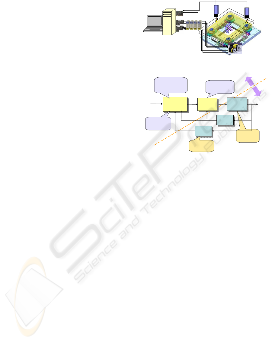
Figure 1 shows the schematic of a PC-based experi-
mental setup for the control of visual alignment sys-
tem. Broadly speaking, it consists of the vision sys-
tem to detect alignment marks on mask and panel
and the stage control system to compensate misalign-
ments. The vision system has normally two CCD
cameras and optical lenses, illumination equipment,
and frame grabber board to capture mark images. In
real production lines, prior to the visual alignment,
the pre-alignment process puts the marks of mask and
panel into the field-of-view of CCD Cameras. Then,
the vision system determines the mark positions in the
global frame and the misalignment distance in camera
coordinate can be converted into the moving distances
of joint actuators through the inverse kinematic solu-
tion of alignment stage.
As denoted in Fig 2, the feedback control system
in the alignment stage has the hierarchical feedback
loops, where the outer visual servoing loop deter-
mines the misalignment quantity between mask and
panel and the inner joint control loop actively com-
pensates it. Due to system uncertainties such as fric-
tion and backlash, the alignment process is usually not
completed by one visual feedback but a few cycles are
repeated.
2.2 Parallel Alignment Stage
As the size of flat panel displays including TFT/LCD,
PDP, and OLED becomes larger and larger, the align-
ment stage is required to have higher load capacity
and wider moving platform. In this regard, the motion
control performance of alignment stage is directly re-
lated to the productivity of the manufacturing process.
Frame
Grabber
DAC
PC processor
CCD/optics/illumination
panel
mask
counter/
decoder
AC servo motor
Figure 1: Schematic of visual alignment control system.
align error
compensation
algorithm
align error
compensation
algorithm
align stage
(UVW)
align stage
(UVW)
vision
system
vision
system
align mark
template
internal
sensor
internal
sensor
feedback
control
feedback
control
sensor fusion
optimal filtering
vision/optics
/illumination
H/W
S/W
pattern recognition
inverse kinematics
trajectory planning
UVW stage
design
precision motion
control design
Figure 2: S/W and H/W components of visual alignment
system.
The advantages of parallel manipulation mechanisms
comparing with serial ones are i) high payload-to-
weight ratio, ii) high structural rigidity since the pay-
load is carried by several limbs, iii) high manipulation
accuracy since active joints are distributed in parallel
and the joint errors are non-cumulative, and iv) sim-
ple inverse kinematic solution. But, they suffer from
smaller workspace and singular configurations. Al-
though the movable range of the parallel stage is very
small (usually a few mms), it is actually enough to
compensate misalignments between mask and panel.
To position the moving platform (in which the
mask is mounted) in a planar location, the task space
of alignment stage must have at least three degrees
of freedom and then it requires at least three active
joints. Hence, it is common for the parallel alignment
stage to have three active limbs. However, if an ex-
tra driving limb is added to support the moving plat-
form, the stiffness and load capacity can be much in-
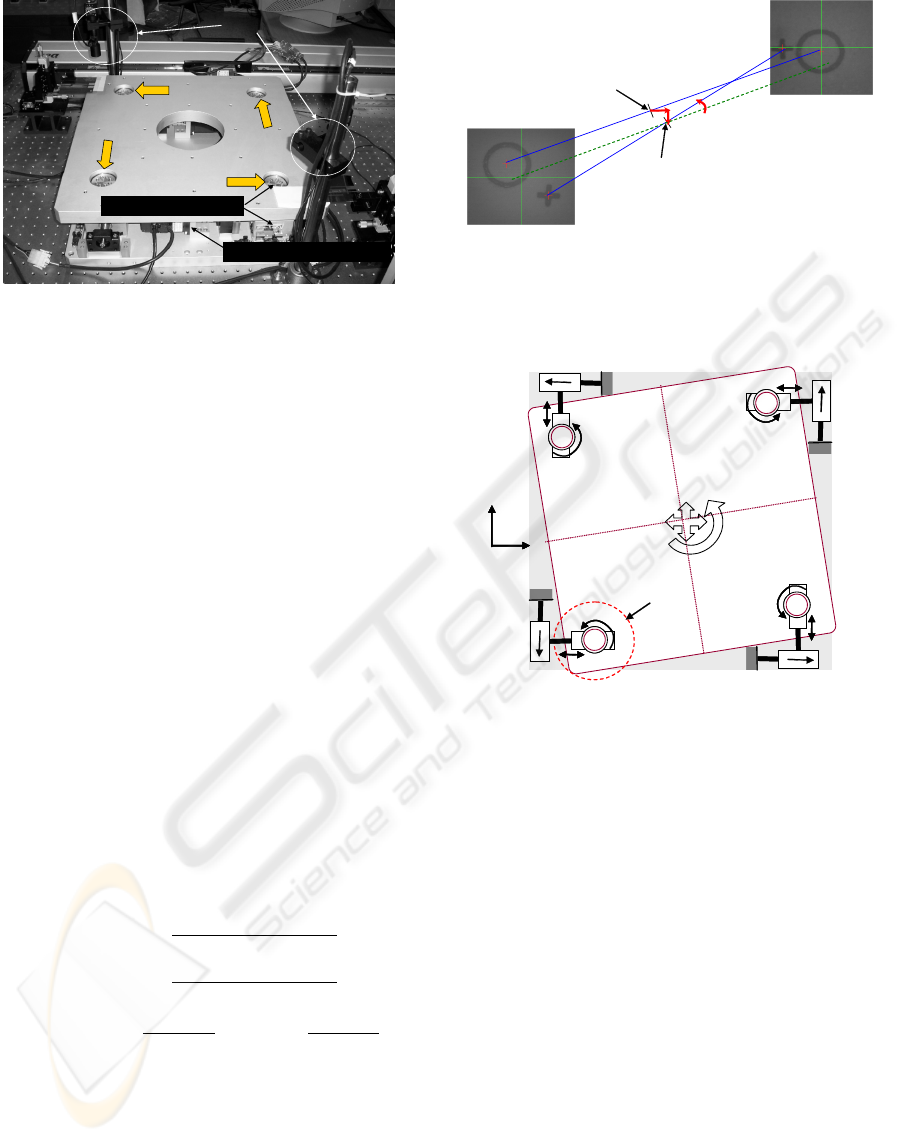
creased. The visual alignment testbed with four driv-
ing axes is shown in Fig. 3, where the motion of the
rotary motor in each limb is transferred to the moving
platform through a ballscrew, cross-roller guide (for
planar translational motion) and cross-roller ring(for
rotational motion).
VISUAL ALIGNMENT ROBOT SYSTEM: KINEMATICS, PATTERN RECOGNITION, AND CONTROL
37
U
V
W
X
CCD
AC servo motor & Ballscrew
Cross roller guide & ring
Moving platform
Figure 3: Visual alignment stage with four active joints.
3 KINEMATICS OF 4PPR
PARALLEL MECHANISM
3.1 Determination of Misalignments
When the centroids of alignment marks of panel and
mask have been obtained through the image process-
ing, it is trivial to get the misaligned posture between
panel and mask. In Fig. 4, let the two align marks
in the panel from the respective CCD image have
the centroids of C
1
= (x
C
1
,y
C
1
) and C
2
= (x
C
2
,y
C
2
)
and those in the mask have L
1
= (x
L
1
,y
L
1
) and L
2
=
(x
L
2
,y
L
2
) in the global frame. Then, the center of line
connecting two centroids can be written as
p
x
= (x
C
1
+ x
C
2
)/2, p
y
= (y
C
1
+ y
C
2
)/2 (1)
for the panel marks and also
m
x
= (x
L
1
+ x
L
2
)/2, m
y
= (y
L
1
+ y
L
2
)/2 (2)
for the mask ones. If the mask is to be aligned to
the panel, the misaligned distance between mask and
panel is given by
∆x = p
x
− m
x
=
x
C
1
− x
L
1
+ x
C
2
− x
L
2
2
(3)
∆y = p
y
− m
y
=
y
C
1
− y
L
1
+ y
C
2
− y
L
2
2
(4)
∆φ = tan
−1
y
C
2
− y
C
1
x
C
2
− x
C
1
− tan
−1
y
L
2
− y
L
1
x
L
2
− x
L
1
(5)
in (x, y) directions and orientation, respectively.
3.2 Mobility of 4ppr Alignment Stage
The degrees of freedom of a mechanism can be found
by the Grubler criterion (Tsai, 1999):
F = λ(n− j − 1) +
∑
i
f
i
− f
p
, (6)
1
L
2
L
2
C
1
C
( , )
M x y
O m m
( , )
P x y
O p p
CCD 1
CCD 2
x∆
y∆
φ
∆
Figure 4: Determination of misaligned posture between
mask and panel (circle: mask marks, cross: panel marks).
x
y
x
y
fixed base
moving platform
PPR joints
U
+
V
+
W+
X
+
Figure 5: Planar 3-DOF, 4PPR parallel mechanim.
where λ is the dimension of the space in which the
mechanism is intended to function, n the number of
links, j the number of joints, f
i
degrees of relative mo-
tion permitted by joint i, and f
p
the passive degrees of
freedom. In the case of a planar 4PPR parallel mech-
anism shown in Fig. 5, in which the moving platform
is supported by four limbs with prismatic-prismatic-
revolute joints, we have λ = 3, n = 2× 4+ 1 + 1 in-
cluding fixed base and moving platform, j = 4 × 3,
∑
f
i
= 12× 1 and f
p
= 0. Hence, the degrees of free-
dom of the 4PPR mechanism is F = 3 as is expected.
In parallel manipulators, every limb forms closed-
loop chain and the number of active limbs is typically
equal to the number of degrees of freedom of the mov-
ing platform. Moreover, each limb has the constraint
of having more joints than the degrees of freedom.
Hence, at least three limbs must have an active joint
(the first P in this case) to achieve the 3-DOF motion
of moving platform and the remaining limb becomes
passive. On the other hand, if all the four limbs are
actuated to increase the rigidity of motion, the actu-
ation redundancy problem is present and a sophisti-
ICINCO 2007 - International Conference on Informatics in Control, Automation and Robotics
38
cated control logic is required to avoid mechanical
singularity.
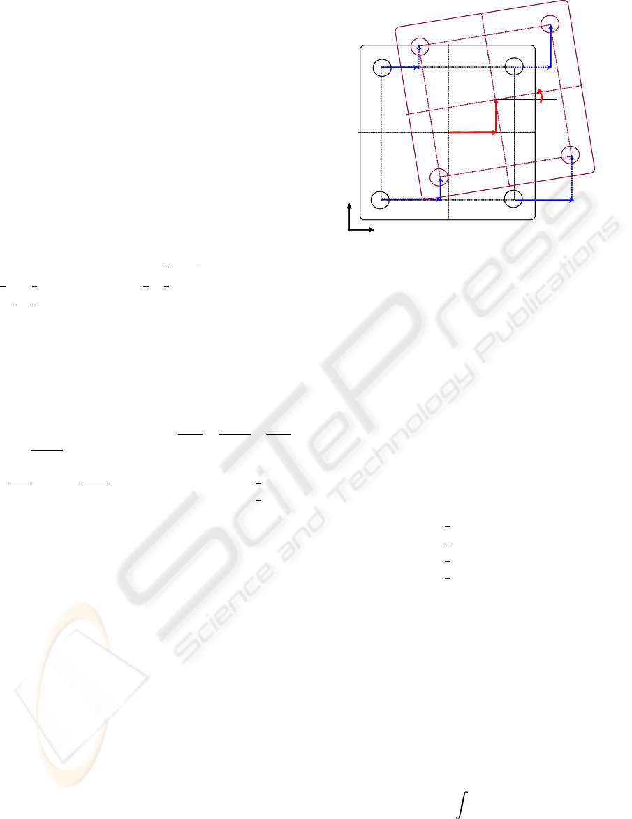
3.3 Inverse Kinematics
The inverse kinematic problem is to seek the moving
ranges of input joints which correspond to the end-
effector movement of a mechanism, i.e., moving plat-
form in this case. In Fig. 6, the square of a fixed base
is defined by the four fixed points (P,Q,R,S) and the
moving platform is connected to the limbs at the four
points (A,B,C, D). We assume that the two squares
have the same side length of h and the global coordi-
nates system is located at the center (O
1
) of the fixed
base.
Then, the positions of fixed points (P, Q, R, S)
are given by (x
P
,y
P
) = (−
1
2
h,−
1
2
h), (x
Q
,y
Q
) =
(
1
2
h,−
1
2
h), (x
R
,y
R
) = (
1
2
h,
1
2
h), and (x
S
,y
S
) =
(−
1
2
h,
1
2
h). Moreover, assuming that the position of
point A in the moving platform is known, the positions
of the other three connecting points can be expressed
as
(x
B
,y
B
) = (x
A
+ hcos∆φ,y
A
+ hsin∆φ) (7)
(x
C
,y
C
) = (x
B
− hsin∆φ,y
B
+ hcos∆φ) (8)
(x
D
,y
D
) = (x
A
− hsin∆φ,y
A
+ hcos∆φ) (9)
In Fig. 6, we have (x
A
,y
A
) =
O
1
A = O
1
O
2
+ O
2
A
where
O
1
O
2
= (∆x,∆y) and
O
2
A = R(∆φ)O
1
P =
cos∆φ − sin∆φ
sin∆φ cos∆φ
−
1
2
h
−
1
2
h
(10)
Hence, the position of point A can be written by the
misalignment variables as
x
A
= ∆x− h(cos∆φ− sin∆φ)/2 (11)
y
A
= ∆y− h(sin∆φ+ cos∆φ)/2 (12)
As denoted in Fig. 6, the moving distances of in-
put prismatic joints have the following relationships
(note the positive directions defined in Fig. 5): U =
x
B
− x
Q
, V = y
C
− y
R
, W = x
S
− x
D
, and X = y
P
− y
A
.
Now, by substituting (7)–(12) into the above expres-
sions, we finally have
U = ∆x+ h(cos∆φ + sin∆φ − 1)/2 (13)
V = ∆y+ h(cos∆φ+ sin∆φ− 1)/2 (14)
W = −∆x+ h(cos∆φ+ sin∆φ− 1)/2 (15)
X = −∆y+ h(cos∆φ+ sin∆φ− 1)/2 (16)
3.4 Forward Kinematics
In serial mechanisms, the inverse kinematic solution
is generally hard to find, but the direct kinematics is
2
O
x
y
x
y
U
V
W
X
x∆
y∆
φ
∆
1
O
A
D
C
B
P
R
Q
S
Figure 6: Moving distances of active (solid line) and pas-
sive (dotted line) joints for a misalignment posture.
straightforward. However, the situation is reversed in
parallel mechanisms, where the inverse kinematics is
rather simple as shown in the former section but the
direct kinematics is more complicated. The inverse
kinematics is important for the control purpose while
the direct kinematics is also required for the kinematic
analysis of end-point.
Although finding out the direct kinematics in po-
sition level could be a long-time procedure, it be-
comes an easy task in velocity level. By differenti-
ating (13)-(16) with respect to the time, the follow-
ing Jacobian relationship between joint space velocity
and task space one is given.
˙
U
˙
V
˙
W
˙
X
=
1 0
1
2
h(cos∆φ− sin∆φ)
0 1
1
2
h(cos∆φ− sin∆φ)
−1 0
1
2
h(cos∆φ− sin∆φ)
0 −1
1
2
h(cos∆φ− sin∆φ)
˙x
˙y
˙
φ
(17)
which can be simply represented by
˙q(t) = J(p) ˙p(t) (18)
Considering the Jacobian J ∈ ℜ
4×3
in (18),
the columns are linearly independent (rank(J)= 3).
Hence, J
T
J ∈ ℜ
3×3
is invertible and there exists a left-
inverse J
+
∈ ℜ
3×4
such that J
+
= (J
T
J)
−1
J
T
and the
linear system (18) has an unique solution ˙p for every
˙q (Strang, 1988). In the sequel, the direct kinematic
solution at current time can be determined by
˙p(t) = J
+
˙q(t) (19)
→ p(t) =
t
t
0
(J
T
J)
−1
J
T
˙q(t)dt (20)
VISUAL ALIGNMENT ROBOT SYSTEM: KINEMATICS, PATTERN RECOGNITION, AND CONTROL
39
4 PATTERN RECOGNITION
A typical visual alignment system provides a struc-
tured vision environment. For example, CCD cam-
era and illumination is under static condition and the
objects to be recognized are just two kinds of align-
ment mark for mask and panel. Moreover, the shape
of marks are usually symmetric ones such as circle,
cross, rectangle, and diamond, in which case the fea-
ture points of an object can be easily determined. We
consider just circle and cross shaped marks because
they are most common in display and semiconductor
industry. In this section, an efficient alignment mark
recognition algorithm in Fig 10 is suggested by com-
bining the conventional labeling technique and a ge-
ometric template matching method which is designed
by analyzing the characteristics of alignment marks, .
Basically, it is assumed that the alignment marks are
in the field-of-view (FOV) of cameras after the pre-
alignment process in the industrial visual alignment
system.
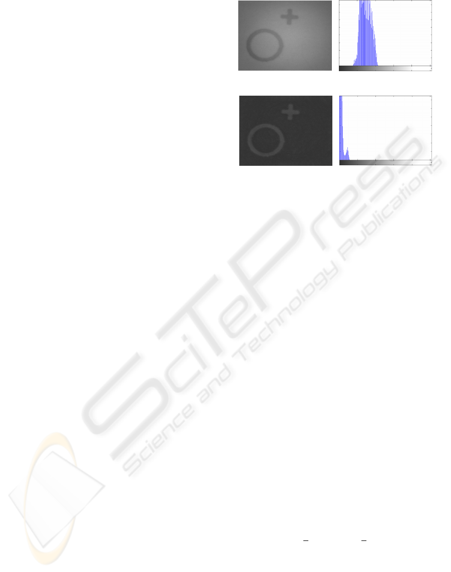
4.1 Preprocessing
Bottom-Hat Transform: Before applying the label-
ing algorithm, the gray image from the CCD cam-
era is converted into the binary image. However, a
proper binarization is impossible when the illumina-
tion is nonlinear or non-steady due to the limit of light
source or other unexpected light disturbances. In or-
der to eliminate these effects, we can use the bottom-
hat transform which is a morphology method (Gonza-
lez and Wood, 2002), where the transformed image h
can be calculated by
h = ( f · b) − f (21)
where f represents the original image, b the circular
morphology, and ( f · b) the closing operation between
f and b. By the closing operation, objects smaller
than the size of b are eliminated and the rest of back-
ground is extracted. The size of b is usually deter-
mined experimentally. The figure 7 shows an exam-
ple.
Dynamic Thresholding and Noise Filtering: To
segregate marks from the background in the Bottom-
Hat transformed image, we apply the binarzation al-
gorithm. Among several methods to determine best
threshold value, the following repetition method can
be used: 1) Set the initial threshold T, which is the
average between the maximum and the minimum of
brightness from the binary image. 2) Divide the im-
age into class G
1
and G
2
by T and calculate the av-
erages m
1
and m
2
of them. 3) Calculate T = (m
1
+
m
2
)/2. 4) Repeat step 2 and step 3 until m
1
and m
2
are not changed.
(a) Original image and the histogram
(b) Bottom-Hat transformed image and the histogram
Figure 7: Comparison of original and transformed image
and the histograms (b = 20 pixels).
Small noise patterns in the binary image can be
recognized as independent areas during the labeling
process. They can be eliminated by the opening and
closing method:
˙
f = ( f ◦ b) · b (22)
where the morphology b is a small (e.g., 3 by 3)
square matrix whose components are all 1, ( f ◦ b) an
opening operator, and
˙
f the filtered image.
Labeling: If the objects in a captured image are
not overlapped, an easily accessible algorithm to ex-
tract them is the labeling technique. To separate
marks from the noise-filtered image, we first apply
the labeling algorithm to the area chained by eight-
connectivity. Once the labeling process is finished,
a number of areas including the marks will be la-
beled. As explained in Fig 10, if the labeled area is
not counted, a new image should be captured by re-
peating the pre-alignment process. If the labeled area
is only one, it is highly possible that two marks are
overlapped and each mark should be extracted by ap-
plying another pattern recognition scheme. If there
are 2 labeled areas, the marks of mask and panel are
not overlapped. Then, the centroids of marks can be
simply calculated by the center of area method:
X
c
=
1
n
n−1
∑
i=0
X
i
, Y
c
=
1
n
n−1
∑
i=0
Y
i
(23)
where X
c
and Y
c
represent the central point of labeled
image and X
i
and Y
i
the horizontal and vertical po-
sitions of the pixels. Finally, if there are more than
3 labeled areas, as denoted in Fig 10, the areas which
have less pixels than a specified number must be elim-
inated through an extra filtering process.
ICINCO 2007 - International Conference on Informatics in Control, Automation and Robotics
40
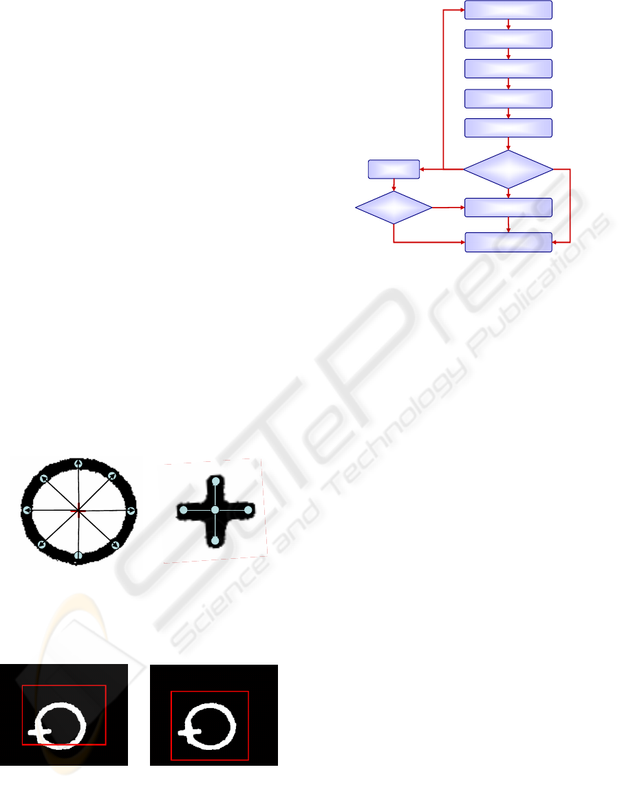
4.2 Geometric Template Matching
When the two marks of mask and panel are over-
lapped, i.e., when the number of labeled area is only
one in Fig 10, the labeling algorithm alone is not
enough but the marks can be separated in terms of
any pattern matching method.
Since the alignment marks used in the display or
semiconductor masks are very simple, their templates
can be readily characterized by a few feature points.
First, for the circular mark in Fig. 8(a) where the ra-
dius (r) is a unique trait, for example, the eight pixels
along the circumference can be selected as the fea-
ture points. All the pixels in the matching area can
be scanned by assuming them as the center of circle.
Then, the centroid of circular mark can be found when
all the feature pixels have the same brightness of 255
(white) in the binarized image. In reality, since the
actual circular mark has a thickness, every pixel that
fulfills this condition must be stored in the memory
stack and the final centroid can be calculated by av-
eraging the coordinate values. Similarly, five feature
points can be chosen for the cross mark with length l
as in Fig. 8(b). However, differently from the circular
mark, we have to consider the rotation factor. Hence,
the matching process should be performed by rotating
the template from 1 to 90 degrees for all pixels in the
matching area.
r
(a) Circular mark
(b) Cross mark
Figure 8: Feature pixels of circular mark (radius = 2 mm)
and cross mark (length = 1 mm).
(a)
(b)
Figure 9: Matching areas for (a) circular mark and (b) cross
mark.
The matching area for the circular mark is given
Pattern matching
Image capture
Bot-Hat transform
Binarization
Noise filtering
Labeling
Calculate centroids
How many
regions?
2
1
over 3
0
How many?
Filtering
2
1
Figure 10: Overall flow of alignment mark recognition.
by the rectangle in Fig. 9(a) with the size of (M −
2r) × (N − 2r) pixels in the M × N pixel image. Un-
der the assumption that the exact central point of the
circular mark has been found, the matching area for
the cross mark is equal to 2(r+ l) × 2(r + l) pixels as
shown in Fig. 9(b) regarding the farthest positions of
the cross mark in the overlapped image.
The normalized correlation (NC) (Manickam
et al., 2000) and the point correlation (PC) algorithm
(Krattenthaler et al., 1994) are most widely used tem-
plate matching methods in machine vision systems.
However, since the NC requires a vector operation
for all pixels in the image and template to determine
the correlation coefficient, it is too time consuming.
Although the PC algorithm reduces the dimension of
computation time, it is still not appropriate for real-
time applications because it includes feature points
extraction process. On the contrary, in our matching
algorithm, the feature points of alignment marks are
geometrically extracted based on the analysis of mark
shape and the individual feature points and the image
pixels at the same coordinates are directly compared
without any vector operations.
The overall sequence of the suggested algorithm
for alignment mark recognition is described in Fig 10,
where the feature pixels of marks can be determined
in advance of labeling and the computation will be
finished at the labeling process when the marks are
not overlapped. As far as the mark shape is geomet-
rically simple, as is the case in semiconductor and
display industry, the combined algorithm of labeling
and geometric pattern matching can be considered as
a reasonable way to reduce the overall tact time.
VISUAL ALIGNMENT ROBOT SYSTEM: KINEMATICS, PATTERN RECOGNITION, AND CONTROL
41
5 CONTROL
The first step in the visual alignment process is to de-
tect the centroids of alignment marks from the raw
images. The visual processing can be divided into
pre-processing and image analysis. As described in
the former section 4, the pre-processing includes bi-
narization, edge detection, and noise filtering etc. In
the image analysis procedure, a few object recogni-
tion techniques can be applied such as labeling and
template matching. Once the centroids of marks are
determined, the misalignment distance and angle be-
tween mask and panel, which is usually less than hun-
dreds of microns, can be readily determined using ge-
ometric relationships. Given the misalignment quan-
tity for the current image, the driving distances of
joint actuators can be produced by the inverse kine-
matic solution for a specific parallel mechanism as
shown in Section 3. Finally, the misalignment can
be compensated by the joint controller as in Fig. 11,
where the outer visual feedback loop should be re-
peated until it meets permissible alignment errors.
Joint
Controller
Inverse
Kinematics
Feature
Extraction
Centroids
Extraction
Misalignment
Determination
Efficient
Image Processing
Efficient
Image Analysis
Fast and Fine
Motion Control
mark images
x 2EA
Figure 11: Vision-based look and move motion control.
XYZ manual
stage
Illumination control
Control PC
Frame
Grabber
Glass mark (d=1mm)
Mask mark (d=2mm)
4PPR stage
CCD 1
CCD 2
CCD Ch. 1
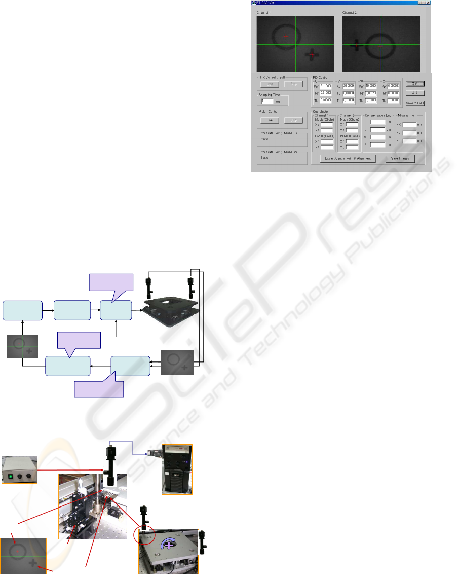
Figure 12: Experimental setup for visual alignment.
Figure 12 shows the experimental setup for the
mask and panel alignment, where the CCD image
Figure 13: Graphic User Interface of operating software.
has the size of 640× 480 pixels and the field of view
(FOV) is 6.4 × 4.8 mm and the rate of capture in the
frame grabber is 15 fps. Circular marks have a diam-
eter of 2 mm and thickness of 200 µm and the cross
marks have the length of 1 mm. The graphic user in-
terface shown Fig. 13 was developed to integrate all
the functions to achieve the autonomous visual align-
ment.
First of all, we compared the performance of the
alignment mark recognition algorithm in Fig. 10
with the popular NC (Manickam et al., 2000) and PC
method (Krattenthaler et al., 1994). For the captured
images in Fig. 13, the proposed method takes 37 msec
on average to find the centroids of all marks including
pre-processing time, while the NC and PC required
661 msec and 197 msec, respectively. As a result,
the proposed method reduces one order of recogni-
tion time. As explained before, this is mainly because
in the geometric template matching the vector oper-
ations for all pixels are not necessary unlike the NC
and the feature points of objects are selected in ad-
vance unlike the PC. Although the geometric pattern
matching is confined to simple objects, it is actually
enough to extract alignment marks.
Figure 14 shows the visual alignment process for
a given misaligned posture between mask and panel.
As explained in Fig. 11, the inverse kinematic solu-
tions are cast into the joint controllers as a reference
input. To avoid excessive chattering, at every align-
ment cycle, we have applied the polynomial trajec-
tory with rise time 0.6 sec for the reference values. In
Fig. 14, the mask and panel were almost aligned after
the 1st cycle and the 2nd cycle was activated since the
misalignments in U-axis and W-axis are still over the
tolerance. Considering the joint control error in Fig.
15 for the 2nd cycle, the controlled motion of V-axis
ICINCO 2007 - International Conference on Informatics in Control, Automation and Robotics
42
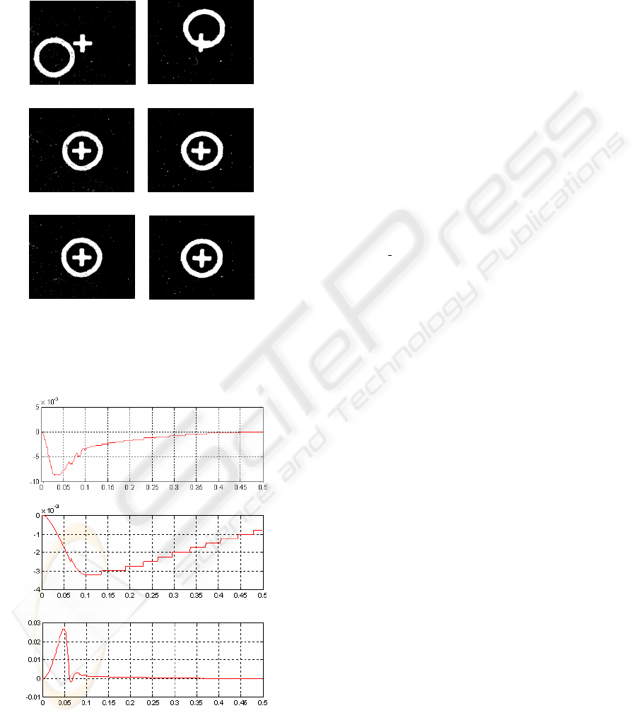
is not smooth. When the reference input is too small,
a stick-slip motion may occur at low velocities and
this makes precision control very difficult.
(a) Initial postures
Ch. 1
Ch. 2
(b) After 1st alignment
(c) After 2nd alignment
Ch. 1
Ch. 2
Ch. 1
Ch. 2
Figure 14: Visual alignment experiment: the inverse kine-
matic solution is (U,V,W) = (132.4, −592.6, −1367.6)µm
at initial posture and (U,V,W) = (−73.4,−3.5, 66.5)µm af-
ter the 1st alignment.
(a) U
-
axis control error
(b) V-axis control error
(b) W-axis control error
mm
mm
mm
time(sec)
time(sec)
time(sec)
Figure 15: Joint control errors during the 2nd alignment
(the 4th X-axis was not active).
6 CONCLUSION
In this paper, we investigated the visual alignment
problem which is considered as a core requirement in
flat panel display and semiconductor fabrication pro-
cess. The kinematics of the 4PPR parallel mechanism
was given and an efficient vision algorithm in terms of
geometric template matching was developed for fast
recognition of alignment marks. Through the control
experiment, the proposed method was proven to be
very effective.
REFERENCES
Cognex Ltd. (2004). In http://www.cognex.com/ prod-
ucts/VisionTools/PatMax.asp.
Gonzalez, R. C. and Wood, R. E. (2002). Digital Image
Processing. Prentice Hall.
Hephaist Ltd. (2004). In http://www.hephaist.co.jp/
e/pro/n
4stage.html.
Kang, D. J. and Lho, T. J. (2003). Development of an edge-
based point correlation algorithm for fast and stable
visual inspection system. In Journal of Control, Au-
tomation and System Engineering. Vol. 9, No. 2, Au-
gust, 2003 (in Korean).
Kanjilal, A. K. (1995). Automatic mask alignment without
a microscope. In IEEE Trans. on Instrumentation and
Measurement. Vol. 44, pp. 806-809, 1995.
Kim, H. T., Song, C. S., and Yang, H. J. (2004). 2-step al-
gorithm of automatic alignment in wafer dicing pro-
cess. In Microelectronics Relaiability. Vol. 44, pp.
1165-1179, 2004.
Krattenthaler, W., Mayer, K. J., and Zeiller, M. (1994).
Point correlation: a reduced-cost template matching
technique. In IEEE Int. Conf. on Image Processing.
pp. 208-212, 1994.
Lai, S.-H. and Fang, M. (2002). A hybrid image alignment
system for fast and precise pattern localization. In
Real-Time Imaging. Vol. 8, pp. 23-33, 2002.
Manickam, S., Roth, S. D., and Bushman, T. (2000). In-
telligent and optimal normalized correlation for high-
speed pattern matching. In Datacube Technical Paper.
Datacube Incorpolation.
Martin, B. R. (2001). Self-alignment of patterned wafers
using capillary forces at a wafer-air interface. In Ad-
vanced Functional Materials. Vol. 11, pp.381-386,
2001.
Strang, G. (1988). Linear Algebra and Its Applications.
College Publishers, 3rd edition.
Tsai, L.-W. (1999). Robot Analysis: The mechanics of se-
rial and parallel manipulators. Wiley-Interscience.
Umminger, C. B. and Sodini, C. G. (1995). An integrated
analog sensor for automatic alignment. In IEEE Trans.
on Solid-State Circuits. Vol. 30, pp. 1382-1390, 1995.
VISUAL ALIGNMENT ROBOT SYSTEM: KINEMATICS, PATTERN RECOGNITION, AND CONTROL
43
