
AN INCREMENTAL MAPPING METHOD BASED ON A
DEMPSTER-SHAFER FUSION ARCHITECTURE
Melanie Delafosse, Laurent Delahoche, Arnaud Clerentin
RTeAM IUT Dpt Informatique, Amiens, France
Anne-Marie Jolly-Desodt
GEMTEX, Roubaix, France
Keywords: Mobile robot localization, 2D-mapping, uncertainty and imprecision modeling.
Abstract: Firstly this article presents a
multi-level architecture permitting the localization of a mobile platform and
secondly an incremental construction of the environment’s map. The environment will be modeled by an
occupancy grid built with information provided by the stereovision system situated on the platform. The
reliability of these data is introduced to the grid by the propagation of uncertainties managed thanks to the
theory of the Transferable Belief Model.
1 INTRODUCTION
Localization and mapping are fundamental problems
for mobile robot autonomous navigation. Indeed, in
order to achieve its tasks, the robot has to determine
its configuration in its environment. But, if this
result is necessary, it is not sufficient. An estimation
of the uncertainty and the imprecision of this
position should be determined and taken into
account by the robot in order to enable it to act in a
robust way and to adapt its behaviour according to
these two values.
The two notions of uncertainty and imprecision
are distinct ones and they m
ust be clearly defined.
The imprecision results from unavoidable
imperfections of the sensors, (ie) the imprecision
representing the error associated to the measurement
of a value. For example, “the weight of the object is
between 1 and 1.5 kg” is an imprecise proposition.
On the other hand, the uncertainty represents the
belief or the doubt we have on the existence or the
validity of a data. This uncertainty comes from the
reliability of the observation made by the system:
this observation can be uncertain or erroneous. In
other words, the uncertainty denotes the truth of a
proposition. For example, “John is perhaps in the
kitchen” is an uncertain proposition.
In a mobile robotics context, these two notions
are pa
ramount. Using several tools and several
localization algorithms, the mobile robot determines
its configuration. Knowing an estimation of the
uncertainty and the imprecision of this computed
localization, it can adopt an adequate behaviour. For
example, if one of these two values is too high, it
would try to improve the localization estimation by
performing a new localization process.
The key tool used in this purpose is the
Transferab
le Belief Model (TBM) (Smets , 1998), a
non-probabilistic variant of the Dempster-Shafer
theory (Shafer, 1976). Indeed, this theory enables to
easily treat uncertainty since it permits to attribute
mass not only on single hypothesis, but also on the
union of hypotheses. We can thus express ignorance.
So it has enabled us to manage and propagate an
uncertainty from low-level data (sensor data) in
order to get a global uncertainty about the robot
localization. We treat the imprecision independently
from the uncertainty because their non-correlation
have been proved in (Clerentin and all., 2003)
Our dual approach is particularly adapted to the
pr
oblem of data integration in an occupancy grid,
used as part of SLAM paradigm.
We can principally find two types of mapping
para
digm to take into account the notion of distance.
The first paradigm consists of computing a cartesian
representation of the environment which generally
used the Extended Kalman filtering (Leonard and
Durrant-Whyte. , 1992). The second approach based
on occupancy grid maps allows to manage the
438
Delafosse M., Delahoche L., Clerentin A. and Jolly-Desodt A. (2007).
AN INCREMENTAL MAPPING METHOD BASED ON A DEMPSTER-SHAFER FUSION ARCHITECTURE.
In Proceedings of the Fourth International Conference on Informatics in Control, Automation and Robotics, pages 438-445
DOI: 10.5220/0001632504380445
Copyright
c
SciTePress
metric maps, which were originally proposed in
(Elfes,1987.) and which have been successfully
employed in numerous mobile robot systems
(Boreinstein and Koren , 1991). In (Fox and
all,1999)
Dieter Fox introduced a general
probabilistic approach simultaneously to provide
mapping and localization. A major drawback of
occupancy grids is caused by their pure sub-
symbolic nature: they provide no framework for
representing symbolic entities of interest such as
doors, desks, etc (Fox and all,1999).
This paper is divided as follows. In a first part,
we will detail how our grid occupancy is presented
and our uncertain and imprecise sensorial model.
Next we will discuss our localization and mapping
method based on beacon recognizing . Finally we
will present the experimental results.
2 PREAMBLE
2.1 Our Grid Occupancy, Its
Initialisation
We choose to model the environment of our mobile
platform with the occupancy grid tool in 2D. Thus,
the error of sensors measure will be implicitly
managed since we will not manipulate a point (x,y)
but a cell of the grid containing an interval of values
([x],[y]). We choose to center the grid with the
initial position of the platform. Then a cell is defined
by its position in the grid . A cell also contains
information concerning its occupancy degree by
some object of the environment. This latter is
defined by a mass function relative to the
discernment frame
Θ1
= {yes, no}. These two
hypotheses respectively correspond to propositions "
yes, this cell is occupied by an object of the
environment " and " no, this cell is not occupied ".
So the mass function of the cell concerning its
occupation is composed of the three values in [0 ,
1], the mass m
cell
(yes) on the hypothesis {yes},
m
cell
(no) on the hypothesis {no} and m
cell
(
Θ1
) on the
hypothesis
{yes
∪
no} representing the ignorance on
its occupancy problem. Initially, we have no a-priori
knowledge of the situation. So to model our total
ignorance, all the cells are initialized with the neutral
mass function , that is to say: m
cell
{yes
∪
no} = 1
and m
cell
{yes} = m
cell
{no} = 0.
2.2 Uncertain and Imprecise Sensorial
Model
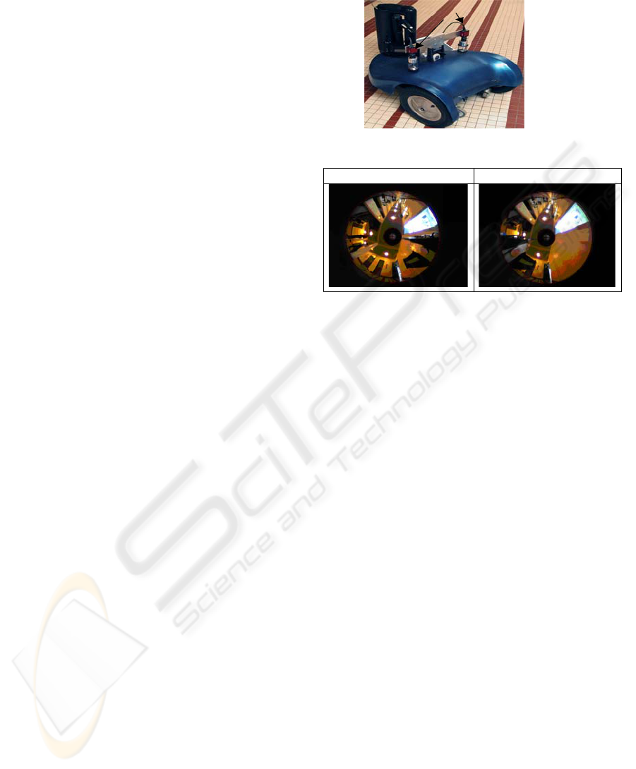
The platform gets a stereovision system composed
of two omnidirectionnal sensors (see
Figure 1.)
distant of about 50 cm. Every acquisition provides
two pictures of the environment .
The two
omnidirectional
vision sensors
Figure 1: The perception system.
Left sensor Right sensor
Figure 2 : An example of an acquisition.
On Figure 2 all vertical landmarks of the
environment like doors or walls project themselves
to the center and form some sectors of different gray
levels. The positions of these landmarks will permit
to fill the occupancy grid and so to build a map . To
get this information, we should associate each sector
in the first picture with the one that corresponds to it
on the second picture. This stage needs some
treatments on the primary data.
First of all, on each omnidirectional picture, we
define a signal which represents the mean RGB
color from a ring localized around the horizon in the
field of view. In fact, what we want to detect are the
natural vertical beacons of the environment.
Omnidirectional vision system project those vertical
parts of the environment according to radial straight
lines onto the image. During this computation, it is
very important that the rings are centered onto the
projection of the revolution axis of the mirror.
Otherwise, we will not compute the mean RGB
color according to the projection of the vertical
elements of the environment. This centering task is
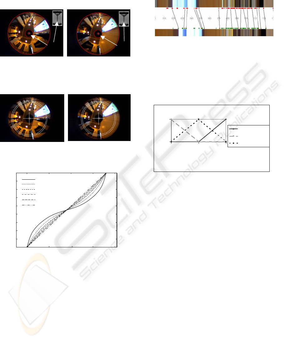
automatically done with a circular Hough transform
(Ballard,1981). In fact, we look for a circle
corresponding to the projection of the black needle
situated onto the top of the hyperbolic mirror (see
Figure 3) which is situated onto the center of the
mirror.
Then, the two 1D mean RGB signals are
computed from the ring(
Figure 4) and matched
together according to a rule of visibility. In fact, if
an object is detected from one omnidirectional
sensor, it will be visible in a certain area of the other
AN INCREMENTAL MAPPING METHOD BASED ON A DEMPSTER-SHAFER FUSION ARCHITECTURE
439
one, according to the distance between the object
and the mobile robot.
Left sensor
The
black
needle
Right sensor
The
black
needle
Figure 3: Center location computed with a circular Hough
transform.
Left sensor Right sensor
Figure 4: Centered rings to compute the mean RGB
signals.
100°
200°
300°
0°
40°
80°
120°
160°
200°
240°
280°
320°
360°
Left
sensor
Right
sensor
0°
35 cm
60 cm
100 cm
150 cm
300 cm
3000 cm
Figure 5: Correspondences between angles from the left
sensor to the right sensor for ob
jects situated at different
distances from the mobile robot.
mobile
rob
could be close to another one. So, we only keep the
Figure 5 shows the correspondences between the
angle of the left sensor and the angle of the right
sensor according to different distances. We actually
notice that the more the object is close to the
ot, the more the two angles are different.
The detection algorithm is based upon the
derivative of the signal in order to detect sudden
changes of color. When we find such value on the
left sensor, we look for a similar change in the right
sensor signal with a maximum of correlation criteria.
In fact, as you can note on the
Figure 6, a matching
most significant matching according to the
correlation value.
Figure 6 : The two extracted mean color signals from
omnidirectional pictures (to 0 from 140°) of
Figure 4 and
the matching between the left sensor (upper) and the right
sensor (bottom).
We choose to use this indicator (in [0-1]) which
qualify a very good correlation when is near than 1,
to build a degree of uncertainty about the matching
by the way of three masses (see
Figure 7 ).
0
1
00,71
absolute correlation coefficent
mass
m(yes)
m(no)
m(yes U no)
Figure 7: Uncertainty about the matching computed with
the correlation coefficient.
When two sectors are matched, we have two
pairs of associated angles on the one hand (angles of
segments that define borders) and on the other hand
a measure of uncertainty on this association. It is
directly linked with a landmark which represents it .
Therefore the pairs define the position of the
landmark and the uncertainty measure its uncertainty
on its existence. So this last value is equal to the set
of three masses coming from the previous fusion in
the discernment frame Θ2= {yes the sectors are
associated; no they do not correspond}
• the mass on the hypothesis “ yes” m
ass
(yes)
• the mass on the hypothesis “ no” m
ass
(no)
the mass on the hypothesis “ I can’t decide about
this matching” m
ass
(yes
∪
no) = m
ass
(
Θ2
) , in other
words this mass represents ignorance.
Then the landmark uncertainty is given by the
following masses in the discernement frame Θ8=
{yes the landmark exist; no it don't exist}:
• the mass on the hypothesis “ yes”
m
land
(yes) = m
ass
(yes)
• the mass on the hypothesis “ no”
m
land
(no) = m
ass
(no)
• the mass on the ignorance hypothesis ie “ I can’t
decide about the existence ”
ICINCO 2007 - International Conference on Informatics in Control, Automation and Robotics
440
m
land
(
Θ8
) =m
ass
(
Θ2
)
Only sectors that have been associated will be
used in the continuation of our survey. The measure
of uncertainty m
land
qualifies the landmark but also
the segment pairs forming borders. Indeed, the
existence of a landmark is linked with the existence
of the borders .
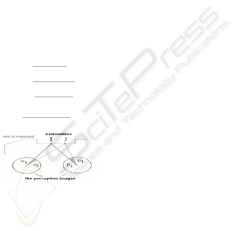
Our data are uncertain but they are also
imprecise because of sensor measurement errors.
This imprecision of measure is managed by the way
of intervals. The second result of this fusion, that is
to say the matching of two angles (
α
,
β
), provides
information about extremities (x
i
, y
i
) of the vertical
landmarks in question(
Figure 8) thanks to equations
of triangulation (1) and (2). So we transform our
data in intervals in order to include this imprecision.
We create a error domain empirically around our
measures of angle (
α , β
). Then the operations (1)
and (2) are computed not between reals but on
intervals . We obtain the following equations (3) and
(4):
ii
i
i
d
x
αβ
β
tantan
tan
−
×
=
(1)
ii
ii
i
d
y
αβ
α
β
tantan
tantan
−
××
=
(2)
[]
[]
[] []
ii
i
i
d
x
αβ
β
tantan
tan
−
×
=
(3)
[]
[] []
[] []
ii
ii
i
d
y
αβ
α
β
tantan
tantan
−
××
=
(4)
Figure 8 : Sectors matching.
At this level of data exploitation, we have a set
of subpaving characterizing the physical extremities
of each landmark detected, that is to say the object
of which sectors representing it have been matched.
These subpavings form the primitive of our sensorial
model that we will try to link with the beacons
during the time. They are localized by their
coordinates ([xi],[yi]) in the frame relative to the
platform and they have the same measure of
reliability that the landmark ie m
prim
= m
land
. .
3 LOCALISATION AND
MAPPING METHOD
The algorithm consists in matching during the
platform displacement the primitives of the sensorial
model with information known from the
environment that we will call beacons. These
matching once achieved will permit both to correct
the position of beacons and the estimated position of
the platform thanks to the odometry and also to
confirm the existence of beacons. In short we will
exploit data of these beacons to build our occupancy
grid of the surrounding space.
3.1 Definition and Initialisation of
Beacon
A beacon is defined by a set of coordinates in the
reference frame (Xe, Ye) (thus forming a subpaving
of localization ) and by a degree of uncertainty about
its existence composed of three masses as previously
shown. This set of masses is established in the
discernment frame
Θ3
={yes , no}. These two
hypotheses respectively correspond to propositions "
yes, this beacon exists " and " no, this beacon does
not exist". So the function mass concerning its
existence is composed of the three values, the mass
m
bea
(yes) on the hypothesis {yes}, m
bea
(no) on the
hypothesis {no} and in short m
bea
(
Θ3
) on the
hypothesis
{yes
∪
no} representing the ignorance
about its existence.
A beacon is born from a primitive observed at
instant t that cannot be matched with the existing
beacons at this instant. This new observation is a
landmark not discovered until now or a false alarm.
The only information on the existence of a new
beacon comes from the existence of the primitive
that gave its birth. Then we choose to give the same
measure of uncertainty on the beacon, that is to say
m
bea t
=m
prim
. Concerning its relative positioning it is
equal to the relative localization subpaving of the
primitive associated. As thereafter we must associate
this beacon to an observation coming from other
acquisitions and should use this one in the updating
of the occupancy grid. So it is more interesting to
manipulate the absolute position . This one is
obtained by the change of a frame in relation to the
configuration of the platform.
Therefore at each instant, new beacons can
appear, and in this case they join the set of the
existing beacons to the following acquisition.
AN INCREMENTAL MAPPING METHOD BASED ON A DEMPSTER-SHAFER FUSION ARCHITECTURE
441
3.2 The Association Method between
Beacons and Primitives
In looking for these matchings, the aim is on the one
hand to get the redundant information permitting to
increase the degree of certainty on the existence of
the beacons and on the other hand to correct their
positioning.
So, at any step, we have several beacons that are
characterized by the center of their subpaving
([x],[y]). Let us call this point the “beacon center”.
The uncertainty of each beacon is represented by the
mass function m
bea t
.
In this part, we try to propagate the matchings
initialised in the previous paragraph with the
observations made during the robot’s displacement.
In other words, we try to associate beacons with
sensed landmarks.
Suppose we manage q beacons at time n. Each
beacon is characterized by its “beacon center”
(expressed in the reference frame). Let us call this
beacon point (x
b
, y
b
). Suppose the robot gets p
observations at time n+1. As we have explained in
the previous paragraph, we are able to compute each
observation localization subpaving ([x
i
], [y
i
]) in the
reference frame. So, for each observation, we have
to search among the q beacons the one that
corresponds to it. In other words, we have to match a
beacon center (x
b
, y
b
) with an observation subpaving
([x
i
], [y
i
]) . The matching criterion we choose is
based on the distance between the beacon center and
the center of observation subpaving ([x
i
], [y
i
]).
So at this level, the problem is to match the p
observations obtained at acquisition n+1 with the q
beacons that exist at acquisition n. To reach this aim,
we use the Transferable Belief Model (Smets, 1998)
in the framework of extended open word (Shafer,
1976) because of the introduction of an element
noted * which represents all the hypotheses which
are not modeled, in the frame of discernment.
First we treat the most reliable primitives, that is
to say the “strong” primitives by order of increasing
uncertainty.
For each sensed primitive Pj (j ∈ [1..p]), we
apply the following algorithm:
– The frame of discernment Θ
j
is composed of:
– the q beacons represented by the hypothesis
Qi (i ∈ [1..q]). Qi means “the primitive Pj is
matched with the beacon Qi”)
– and the element * which means “the primitive
Pj cannot be matched with one of the q
beacons”.
– So: Θ
j
={Q
1
, Q
2
, …, *}
– The matching criterion is the distance between
the center of the subpaving of observation Pj and
one of the beacon centers of Qi
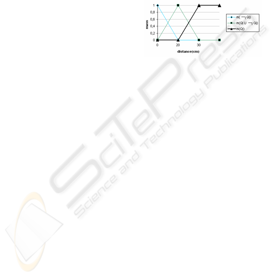
– Considering the basic probability assignment
(BPA) shown
Figure 9, for each beacon Qi we
compute:
– m
i
(Qi) the mass associated with the
proposition “Pj is matched with Qi”.
– m
i
(¬Qi) the mass associated with the
proposition “Pj is not matched with Qi”.
– m
i
(Θ
j
) the mass representing the ignorance
concerning the observation Pi.
– The BPA is shown on Figure 9.
Figure 9: BPA of the matching criterion.
– After the treatment of all the q beacons, we have
q triplets :
– m
1
(Q
1
) m
1
(¬Q
1
) m
1
(Θ
j
)
– m
2
(Q
2
) m
2
(¬Q
2
) m
2
(Θ
j
)
– …
– m
q
(Q
q
) m
q
(¬Q
q
) m
q
(Θ
j
)
– We fuse these triplets using the disjunctive
conjunctive operator built by Dubois And Prade
(Dubois and Prade, 1998). Indeed, this operator
allows a natural conflict management, ideally
adapted for our problem. In our case, the conflict
comes from the existence of several potential
candidates for the matching, that is to say some near
beacons can correspond to a sensed landmark. With
this operator, the conflict is distributed on the union
of the hypotheses which generate this conflict.
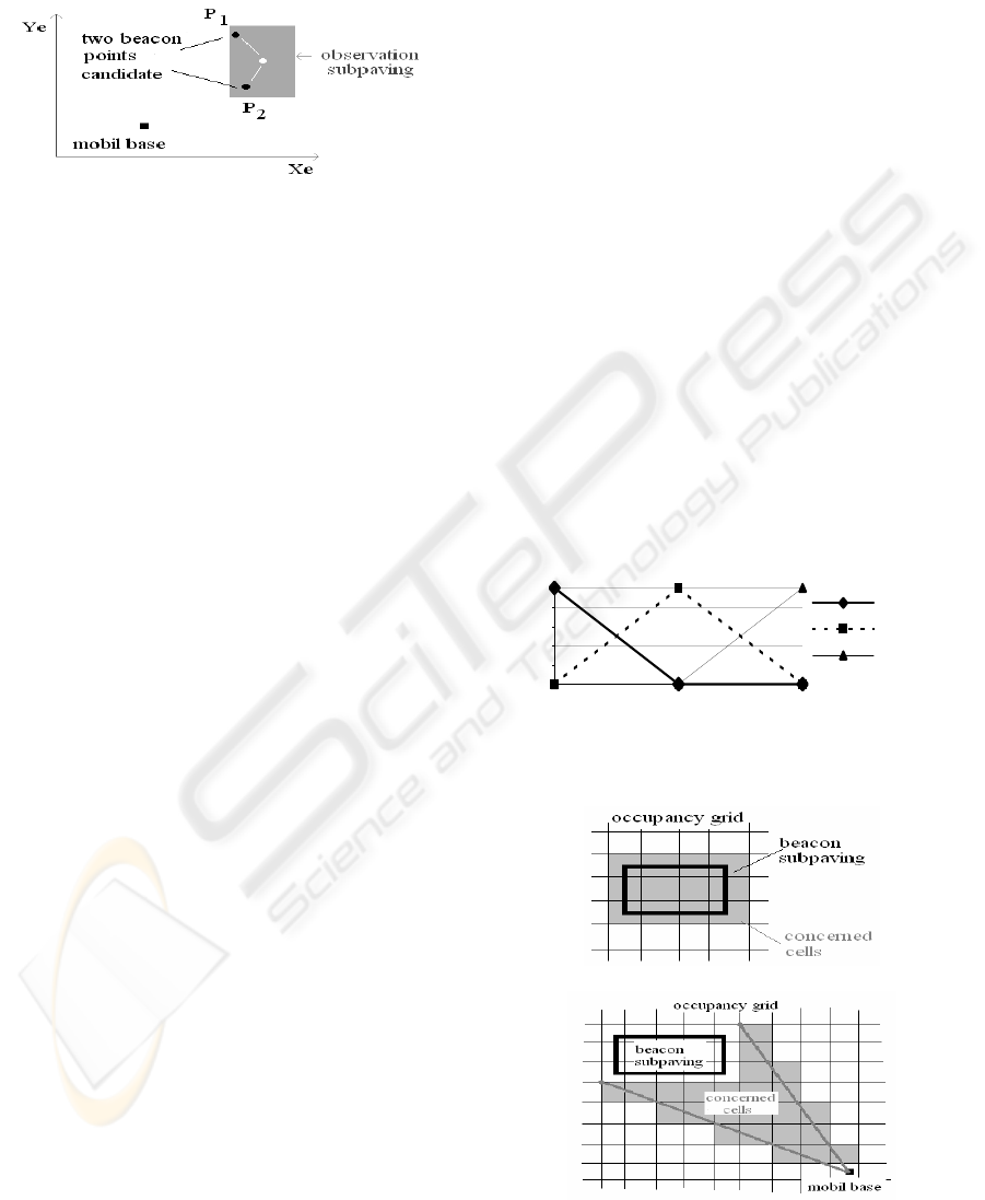
For example, on
Figure 10 , the beacon center P
1
and P
2
are candidates for a matching with the
primitive subpaving ([x], [y]). So m
1
(P
1
) is high (the
expert concerning P
1
says that P
1
can be matched
with ([x], [y])) and m
2
(P
2
) is high too. If the fusion is
performed with the classical Smets operator, these
two high values produce some high conflict. But,
with the Dubois and Prade operator, the conflict
generated by the fusion of m
1
(P
1
) and m
2
(P
2
) is
rejected on m
12
(P
1
∪ P
2
). This means that both P
1
and P
2
are candidates for the matching.
– So, after the fusion of the q triplets with this
operator, we get a mass on each single hypothesis
m
match
(Qi), i ∈ [1..q], on all the unions of hypotheses
m
match
(Qi ∪ Qj…∪ Qq), on the star hypothesis
m
match
(*) and on the ignorance m
match
(Θ
j
).
– The final decision is the hypothesis which has
the maximal pignistic probability (Smets, 1998). If it
is the * hypothesis, no matching is achieved. This
ICINCO 2007 - International Conference on Informatics in Control, Automation and Robotics
442
situation can correspond to two cases: either the
primitive Pj is an outlier, or Pj can be used to initiate
a new beacon since any existing track can be
associated to it.
Figure 10: An example of two beacons that generate some
conflict.
Once a matching is achieved, the uncertainty of
the concerned beacon has to be updated. This
uncertainty is denoted by the mass function m
bea
defined on the frame of discernment Θ
3
. This
updating has to take the reliability of the matched
primitive (mass function m
prim
) and also the
uncertainty of the matching into account. This
matching uncertainty is deduced from the pignistic
probability of the selected matched primitive by the
mass function m2 shown on
Figure 11. For example,
if the pignistic probability is equal to 0.75, the
matching uncertainty is denoted by the following
mass function m
2
: m
2
(yes)=m
2
({yes, no})=0.5 ;
m
2
(no)=0.
Finally, the beacon uncertainty at time t (denoted
by the mass function m
bea t
) is updated by fusing the
beacon uncertainty at the previous time t-1, the
primitive uncertainty (m
prim
) and the matching
uncertainty (m
2
): m
bea t
= m
bea t-1
∩ m
prim
∩ m
2
,
where ∩ is the fusion operator of Smets.
Let us recall that this mass function is composed
of three values: m
bea t
(yes), m
bea t
(no), m
bea t
(Θ
3
).
3.3 The Management of non Associated
Beacons
Concerning the beacons that have not been matched
at this instant, our first reflection was the following.
As no observation can be associated, it implies that
our beacon has not been detected to this acquisition.
Therefore the first idea was to put in doubt its
existence in decreasing its degree of existence. But
even if the beacon is no more visible from instant t
for example because the mobile platform is moving ,
the object nevertheless exists. It is necessary not to
lose this information at the level of the map. Then
we decide not to modify the degree of existence of a
beacon which was not matched.
3.4 The Consequences on our Grid
A new beacon or a beacon that have been associated
to an observation provide two kinds of information
both on the occupied space and on the empty space
of our grid. Let us examine the case of one of these
beacons at time t to explain this phenomenon. As we
have already said, this beacon has a measure of
uncertainty on its existence. It is defined by the mass
function m
bea t
.
3.4.1. The Occupied Space
The existence of a beacon is directly bound to the
occupation of cells containing its localization
subpaving. Therefore the degree of occupation of
these cells must take the degree of existence of the
beacon into account. It is achieved thanks to the
fusion with the operator of Smets of these two mass
functions. So if the mass function of the beacon
indicates rather a certain existence then this fusion
will increase the degree of occupation of concerned
cells. On the contrary, if it indicates an existence
which is somewhat unreliable, the fusion will
reverberate this doubt on these same cells. A cell is
concerned by the fusion if its intersection with the
localization subpaving is not empty, they appear in
gray on
Figure 12a.
0
0.2
0.4
0.6
0.8
1
00.51
maximal pignistic probabililty
mass
m( NO)
m({YES,NO})
m(YES)
Figure 11: Mass function m2 of the matching uncertainty.
Figure 12: a) Occupied Space, b) Free Space.
AN INCREMENTAL MAPPING METHOD BASED ON A DEMPSTER-SHAFER FUSION ARCHITECTURE
443

The fusion is the following:
m
cell t
= m
cell t-1
∩ m
bea t
3.4.2 The Free Space
On the other hand, since this beacon has been
associated to an observation, it implies that the space
between the point of observation in this case the
mobile platform and the beacon does not contain any
obstacle. This space is therefore free. But it is free in
relation with the existence of the beacon.
This operation is achieved in the same way as
previously, that is to say merging with the operator
of Smets. But this time, we fuse its current
occupation degree with a mass function m
3
built as
being the “contrary” of the mass function m
bea t
.
Because the more the beacon is denoted by a high
mass on the hypothesis {yes, I exist} , the more the
mass on the hypothesis {no, this cell is not
occupied} for the cell of the free space (
Figure 12 b)
must increase . This function m
3
is the next one:
m
3
{ no} = m
bea t
{yes}, m
3
{ yes ∪ no} = m
bea t
{
yes ∪ no} and m
3
{yes} = m
bea t
{ no}.
And this fusion is given by the following
expression : m
cell t
= m
cell t-1
∩ m
3
To resume we get a set of beacons and a
occupancy grid of obstacles of the surrounding
space.
3.5 The Correction Method
Now we use these data to correct the position of
beacons at first and then the estimated position of
the mobile platform . These stages are under
development. We currently use the correction
modules presented below that will be to improve in
future works. The beacons are characterized by an
error domain of center (x,y). We notice that this
center, disposed on the grid, is surrounded with the
cells of different occupation levels. To take account
of the information we modify the position of the
beacon. In fact, we choose the center of gravity of a
window 5 x 5 cells around the center pondered by
their respective mass m
cell
(yes) , as the point that
now characterizes the position of the beacon.
Let us remember that the configuration of the
mobile platform is estimated with odometric
information. Or we know the classical phenomena of
cumulative error if no correction method is achieved
(Delafosse and all , 2005). Our correction module is
based on the cumulative error minimization. We
limit the real possible positions of the platform to
centers of cells of a window 3 x 3 around the
position estimated by odometry. The kept position
among the nine will be the p position that minimizes
the accumulated sum of distances between beacons
and primitives observed since the p position.
4 EXPERIMENTAL RESULTS
We present experimental results obtained in a
structured indoor environment on
Figure 13 . The
platform is stopped to every stereoscopic acquisition
achieved every 30 cms. The managed trajectory is a
large boucle represented in yellow on the
Figure 14.
The natural landmarks mainly observed are the
framings of doors, corners , walls and pillars .In
Figure 14 we present the obtained map building. The
blue cells correspond to the empty space and the red
one to the occupied space. The intermediate colors
highlight the merging of the occupied and free state.
We can notice that the method is robust since most
observable landmarks are integrated to the map
according to the real map presented in grey on the
graphs. We can easily detect for example the corners
of the “cross” hall and the free space between each
others. We can also notice the certainty of the free
space is clearly represented by the color purple. Our
approach complementary to the probabilistic one,
form an alternative to the SLAM paradigm based on
the occupancy grid. We can observe the correlation
between the uncertainty of a landmark position
estimation and the updating cell values.
5 CONCLUSION
In this article we have presented an architecture of
fusion and integration of data for the SLAM
paradigm. It is based on a representation of
occupancy grid type. The originality of the
proposition is on the one hand the propagation of
uncertainties on several levels of treatments and on
the other hand the management uncoupled of
imprecision and uncertainty. The association of
these two concepts permits an important reliability
in the process of new primitive integrations in the
map. This step is crucial since it conditions the
global consistency of the cartographic representation
on an important number of acquisitions. Moreover
our approach permits to solve the problem of
“primitive number explosion” which generally
implies a divergence of the SLAM process. Besides
the precision obtained on the position estimation of
observable landmarks is relatively important. So the
«symbolic» approach presented constitutes an
interesting alternative to methods classically used in
this domain that are generally probabilistic.
ICINCO 2007 - International Conference on Informatics in Control, Automation and Robotics
444
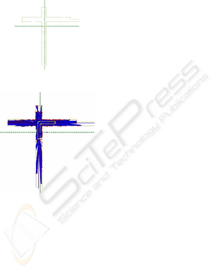
Figure 13: The experimental environment (scale 1m x
1m). We focus on the part of the corridor which represente
a cross.
Figure 14 : The resulting map.
REFERENCES
Ballard D. H., "Generalizing the Hough transform to
detect arbitrary shapes."
Pattern Recognition, v. 13, n.
2, pp. 111-122, 1981.
Boreinstein J. , Koren Y., 1991. “Histogrammic in-motion
mapping for mobile robot obstacle avoidance”, IEEE
Trans. On rob. and auto., Vol. 7, N°4, pp. 1688-1693
Clerentin A., Delahoche L., Brassart E., Drocourt C.,
2003. "Uncertainty and error treatment in a dynamic
localization system", proc. of the 11th Int. Conf. on
Advanced Robotics (ICAR03), pp.1314-1319,
Coimbra, Portugal.
Delafosse M., Clerentin C., Delahoche L., Brassart E.,
2005. “Uncertainty and Imprecision Modeling for the
Mobile Robot Localization Problem” – IEEE
international conference on robotics and automation
ICRA 05 , Barcelona, Spain.
Dubois D., Prade H., Sandri S., 1998. Possibilistic logic
with fuzzy constants and fuzzily restricted quantifiers.
In: Logic Programming and Soft Computing,
(Martin,T.P. et Arcelli-Fontana,F., Eds.), Research
Studies Press, Baldock, England, 69-90.
Elfes A. 1987. “Sonar-based real world mapping and
navigation”, IEEE Journal of robotics and automation,
Vol. RA-3, N°3, pp. 249-265, June 1987
Fox D., Burgard W. , Thrun S. ,1999. "Probabilistic
Methods for Mobile Robot Mapping", Proc. of the
IJCAI-99 Workshop on Adaptive Spatial
Representations of Dynamic Environments.
Leonard J.J., Durrant-Whyte H.F. , 1992. “Dynamic map
building for an autonomous mobile robot”, The
International Journal of Robotics Research, Vol. 11
n°4, August
Royère C, 2002. “Contribution à la résolution du conflit
dans le cadre de la théorie de l’évidence”, thèse de
doctorat de l’Université de Technologie de
Compiègne.
Shafer GA, 1976. A mathematical theory of evidence,
Princeton : university press.
Smets Ph ,1998. “The Transferable Belief Model for
Quantified Belief Representation.”, Handbook of
Defeasible Reasoning and Uncertainty Management
Systems, Kluwer Ed, pp 267-301.
AN INCREMENTAL MAPPING METHOD BASED ON A DEMPSTER-SHAFER FUSION ARCHITECTURE
445
