
EXPLICIT PREDICTIVE CONTROL LAWS
On the Geometry of Feasible Domains and the Presence of Nonlinearities
Sorin Olaru, Didier Dumur
Automatic Control Department, Sup
´
elec, 3 rue Joliot Curie, Gif-sur-Yvette, France
Simona Dobre
CRAN, Nancy - Universit
´
e, CNRS UMR 7039, BP 239, F-54506 Vandœuvre-l
`
es-Nancy Cedex, France
Keywords:
Predictive control, parameterized polyhedra, explicit control laws.
Abstract:
This paper proposes a geometrical analysis of the polyhedral feasible domains for the predictive control laws
under constraints. The fact that the system dynamics influence the topology of such polyhedral domains is
well known from the studies dedicated to the feasibility of the control laws. Formally the system state acts as a
vector of parameters for the optimization problem to be solved on-line and its influence can be fully described
by the use of parameterized polyhedra and their dual constraints/generators representation.
Problems like the constraints redundancy or the construction of the associated explicit control laws at least for
linear or quadratic cost functions can thus receive fully geometrical solutions. Convex nonlinear constraints
can be approximated using a description based on the parameterized vertices. In the case of nonconvex re-
gions the explicit solutions can be obtain by constructing Voronoi partitions based on a collection of points
distributed over the borders of the feasible domain.
1 INTRODUCTION
The philosophy behind Model-based Predictive Con-
trol (MPC) is to exploit in a ”receding horizon” man-
ner the simplicity of the Euler-Lagrange approach
for the optimal control. The control action u
t
for a
given state x
t
is obtained from the control sequence
k
∗
u
= [u
T
t
,...,u
T
t+N−1
]
T
as a result of the optimization
problem:
min
k
u
ϕ(x
t+N
) +
N−1
∑
k=0
l(x
t+k
,u
t+k
)
subj.to : x
t+1
= f(x
t
) + g(x
t
)u
t
;
h(x
t
,k
u
) ≤ 0
(1)
constructed for a finite prediction horizon N, cost per
stage l(.), terminal weight ϕ(.), the system dynam-
ics described by f(.), g(.) and the constraints written
in a compact form using elementwise inequalities on
functions linking the states and the control actions,
h(.).
Unfortunately, the control sequence k
∗
u
is optimal
only for a single initial condition - x
t
and produces
an open-loop trajectory which contrasts with the need
for a feedback control law. This drawback is over-
come by solving the local optimization (1) for ev-
ery encountered (measured) state, thus indirectly pro-
ducing a state feedback law. The overall method-
ology is based on computationally tractable optimal
control problems for the states found along the cur-
rent trajectory. However, two important directions
are to be studied in order to enlarge the class of sys-
tems which can take advantage of the MPC method-
ology. One is related to the fact that the measure-
ments can be available faster than the optimal con-
trol sequence becomes available (as output of the op-
timization solver) and thus important information can
be lost with irreversible consequences on the close-
loop performances. Secondly, the lack of a closed
form expression for the feedback law notifies about
the difficulties that can be encountered when consid-
ering properties such as stability, typically established
for regions in the state space.
For the optimization problem (1) within MPC, the
current state serves as an initial condition and in-
fluences both the objective function and the feasible
domain. Globally, from the optimization point of
view, the system state can be interpreted as a vec-
tor of parameters, and the problems to be solved
70
Olaru S., Dumur D. and Dobre S. (2007).
EXPLICIT PREDICTIVE CONTROL LAWS - On the Geometry of Feasible Domains and the Presence of Nonlinearities.
In Proceedings of the Fourth International Conference on Informatics in Control, Automation and Robotics, pages 70-77
DOI: 10.5220/0001633200700077
Copyright
c
SciTePress

are part of the multiparametric optimization program-
ming family. From the cost function point of view,
the parametrization is somehow easier to deal with
and eventually can be entirely translated towards the
set of constraints to be satisfied (the MPC literature
contains references to schemes based on suboptimal-
ity or even to algorithms restraining the demands to
feasible solution of the receding horizon optimization
(Scokaert et al., 1999)). Unfortunately, similar obser-
vation cannot be made about the feasible domain and
its adjustment with respect to the parameters evolu-
tion.
The optimal solution is often influenced by the
limitations, the process being forced to operate at the
designed constraints for best performance. The dis-
tortion of the feasible domain during the parameters
evolution will consequently affect the structure of the
optimal solution. Starting from this observation the
present paper focuses on the topological analysis of
the domains described by the MPC constraints.
The structure of the feasible domain is depending
on the model and the set of constraints taken into con-
sideration in (1). If the model is a linear system, the
presence of linear constraints on inputs and states can
be easily expressed by a system of linear inequalities.
In the case of nonlinear systems, these properties are
lost and the domains are in general difficult to han-
dle. However, there are several approaches to trans-
form the dynamics to those of a linear system over
the operating range as for example by piecewise lin-
ear approximation, feedback linearisation or the use
of time-varying linear models.
As a consequence, specific attention for the lin-
ear constraints and the associated polyhedral feasi-
ble domains may be prolific. More than that, the
use of polyhedral domains between the convex sets is
not hazardous since they offer important advantages,
like the closeness over the intersection or the fact that
the polyhedral invariant sets (largely used for enforc-
ing stability) are less conservative than the ellipsoidal
ones for example. In the current paper, these polyhe-
dral feasible domains will be analyzed with a focus on
the parametrization leading to the concept of parame-
terized polyhedra (Olaru and Dumur, ):
min
k
u
F(x
t
,k
u
)
subj.to :
A
in
k
u
≤ b
in
+ B
in
x
t
A
eq
k
u
= b
eq
+ B
eq
x
t
h(x
t
,k
u
) ≤ 0
(2)
where the objective function F(x
t
,k
u
) is usually lin-
ear or quadratic.
Secondly it will be shown that the optimization
problem may take advantage during the real-time im-
plementation either from the possible alleviation of
the set of constraints for the on-line optimization rou-
tines either from the construction of the explicit solu-
tion on geometrical basis when possible. With these
two aspects, one can consider that MPC awareness
is improved both from the theoretical (insight on the
global control law) and practical (computational as-
pects) point of view.
An important remark concerning the presence of
nonlinearities in the constraints is that if the feasi-
ble domain remains convex, then an approximation in
terms of parameterized polyhedra can lead to an ap-
proximate explicit solution in terms of piecewise lin-
ear control laws. But, if the feasible domain becomes
non-convex due to the presence of nonlinearities, then
in order to obtain the explicit solution some assump-
tion have to be relaxed. A special role, in finding the
explicit control laws in the nonlinear case, is played
by the Voronoi partition.
In the following, Section 2 introduces the basic
concepts related to the parameterized polyhedra and
interprets the feasible domains of the receding hori-
zon optimization problems (2) in this context. Sec-
tion 3 presents the use of the feasible domain analysis
for the construction of the explicit solution for linear
and quadratic objective functions. In Section 4 an ex-
tension to nonlinear type of constraints is addressed,
simple examples illustrating the construction of ex-
plicit solutions.
2 PARAMETRIZATION OF
POLYHEDRAL DOMAINS
2.1 Double Representation
A mixed system of linear equalities and inequalities
defines a polyhedron (Motzkin and R.M., 1953). In
the parameter free case, it is represented by the equiv-
alent dual (Minkowski) formulation:
P =
k
u
∈ R
p
A
eq
k
u
= b
eq
;A
in
k
u
≤ b
in
⇐⇒
P = conv.hullV+ coneR+ lin.spaceL
|
{z }
generators
(3)
where conv.hullV denotes the set of convex combi-
nations of vertices V =
{
v
1
,...,v
ϑ
}
, coneR denotes
nonnegative combinations of unidirectional rays
in R =
r
1
,...,r
ρ
and lin.spaceL =
{
l
1
,...,l
λ
}
represents a linear combination of bidirectional rays
(with ϑ, ρ and λ the cardinals of the related sets).
This dual representation (Schrijver, 1986) in terms of
generators can be rewritten as:
EXPLICIT PREDICTIVE CONTROL LAWS - On the Geometry of Feasible Domains and the Presence of Nonlinearities
71

P =
k
u
∈ R
p
|
k
u
=
ϑ
∑
i=1
α
i
v
i
+
ρ
∑
i=1
β
i
r
i
+
λ
∑
i=1
γ
i
l
i
;
0 ≤ α
i
≤ 1,
ϑ
∑
i=1
α
i
= 1 , β
i
≥ 0 , ∀γ
i
(4)
with α
i
, β
i
, γ
i
the coefficients describing the convex,
non-negative and linear combinations in (3).
Numerical methods like the Chernikova algorithm
(Leverge, 1994) are implemented for constructing the
double description, either starting from constraints (3)
either from the generators (4) representation.
2.2 The Parametrization
A parameterized polyhedron (Loechner and Wilde,
1997) is defined in the implicit form by a finite num-
ber of inequalities and equalities with the note that the
affine part depends linearly on a vector of parameters
x ∈R
n
for both equalities and inequalities:
P (x) =
k
u
(x) ∈ R
p
A
eq
k
u
= B
eq
x+ b
eq
;
A
in
k
u
≤ B
in
x+ b
in
}
=
k
u
(x)
|
k
u
(x) =
ϑ
∑
i=1
α
i
(x)v
i
(x)
+
ρ
∑
i=1
β
i
r
i
+
λ
∑
i=1
γ
i
l
i
0 ≤ α
i
(x) ≤ 1,
ϑ
∑
i=1
α
i
(x) = 1 , β
i
≥ 0 , ∀γ
i
.
(5)
This dual representation of the parameterized poly-
hedral domain reveals the fact that only the vertices
are concerned by the parametrization (resulting the
so-called parameterized vertices - v
i
(x)), whereas the
rays and the lines do not change with the parame-
ters’ variation. In order to effectively use the gener-
ators representation in (5), several aspects have to be
clarified regarding the parametrization of the vertices
(see for exemple (Loechner and Wilde, 1997) and the
geometrical toolboxes like POLYLIB (Wilde, 1993)).
The basic idea is to identify the parameterized polyhe-
dron with a non-parameterized one in an augmented
space:
˜
P =
k
u
x
∈ R
p+n
|
A
eq
−B
eq
k
u
x
= b
eq
;
[A
in
|
−B
in
]
k
u
x
≤ b
in
(6)
The original polyhedron in (5) can be found for
any particular value of the parameters vector x
through P(x) = Proj
k
u
˜
P∩H(x)
, for any given hy-
perplane H(x
0
) =
k
u
x
∈ R
p+n
|
x = x
0
and
using Proj
k
u
(.) as the projection from R
p+n
to the first
p coordinates R
p
.
Within the polyhedral domains
˜
P , the correspon-
dent of the parameterized vertices in (5) can be found
among the faces of dimension n. After enumerating
these n-faces:
n
F
n
1
(
˜
P ),...F
n
j
(
˜
P ),...,F
n
ς
(
˜
P )
o
, one
can write: ∀i, ∃j ∈
{
1,...,ς
}
s.t.
v
i
(x)
T
x
T
T
∈
F
n
j
(
˜
P ) or equivalently:
v
i
(x) = Proj
k
u
F
n
j
(
˜
P ) ∩H(x)
(7)
From this relation it can be seen that not all the n-
faces correspond to parameterized vertices. However
it is still easy to identify those which can be ignored
in the process of construction of parameterized ver-
tices based on the relation: Proj
x
F
n
j
(
˜
P)
< n with
Proj
x
(.) the projection from R
p+n
to the last n coor-
dinates R
n
(corresponding to the parameters’ space).
Indeed the projections are to be computed for all the
n-faces, those which are degenerated are to be dis-
carded and all the others are stored as validity do-
mains - D
v
i
∈ R
n
, for the parameterized vertices that
they are identifying:
D
v
i
= Proj
n
F
n
j
(
˜
P)
(8)
Once the parameterized vertices identified and their
validity domain stored, the dependence on the param-
eters vector can be found using the supporting hyper-
planes for each n-face:
v
i
(x) =
A
eq
¯
A
in
j
−1
B
eq
¯
B
in
j
x+
b
eq
¯
b
in
j
(9)
where
¯
A
in
j
,
¯
B
in
j
,
¯
b
in
j
represent the subset of the in-
equalities, satisfied by saturation for F
n
j
(
˜
P). The in-
version is well defined as long as the faces with de-
generate projections are discarded.
2.3 The Interpretation from the
Predictive Control Point of View
The double representation of the parameterized poly-
hedra offers a complete description of the feasible do-
main for the predictive control law as long as this is
based on a multiparametric optimization with linear
constraints.
Using the generators representation, with simple
difference operations on convex sets one can compute
the region of the parameters space where no parame-
terized vertex is defined:
ℵ = R
n
\
{
∪D
v
i
; i = 1...ϑ
}
(10)
representing from the MPC point of view, the set of
infeasible states for which no control sequence can be
designed due to the fact that the limitations are overly
ICINCO 2007 - International Conference on Informatics in Control, Automation and Robotics
72

constraining. As a consequence the complete descrip-
tion of the infeasibility is obtained.
Remark: the presence of rays and lines in the set
of generators doesn’t imply that the infeasibility is
avoided. The feasibility is strictly related with the ex-
istence of valid parameterized vertices for the given
value of the parameter (state) vector.
The vertices of the feasible domain cannot be
expressed as convex combinations of other distinct
points and, due to the fact that from the MPC point
of view, they represent sequences of control actions,
one can interpret them in terms of extremal perfor-
mances of the controlled system (for example in the
tracking applications the maximal/minimal admissi-
ble setpoint (Olaru and Dumur, 2005)).
3 TOWARDS EXPLICIT
SOLUTIONS
In the case of sufficiently large memory resources,
construction of the explicit solution for the multipara-
metric optimization problem can be an interesting al-
ternative to the iterative optimization routines. In this
direction recent results where presented at least for
the case of linear and quadratic cost functions (see
(Seron et al., 2003),(Bemporad et al., 2002),(Good-
win et al., 2004),(Borelli, 2003),(Tondel et al., 2003)).
In the following it will be shown that a geometrical
approach based on the parameterized polyhedra can
bring a useful insight as well.
3.1 Linear Cost Function
The linear cost functions are extensively used in con-
nection with model based predictive control and espe-
cially for robust case ((Bemporad et al., 2001), (Ker-
rigan and Maciejowski, 2004)). In a compact form,
the multiparametric optimization problem is:
k
u
∗
(x
t
) = min
k
u
f
T
k
u
subject to A
in
k
u
≤ B
in
x
t
+ b
in
(11)
The problem deals with a polyhedral feasible do-
main which can be described as previously in a dou-
ble representation. Further the explicit solution can
be constructed based on the relation between the pa-
rameterized vertices and the linear cost function (as in
(Leverge, 1994)). The next result resumes this idea.
Proposition: The solution for a multiparametric
linear problem is characterized as follows:
a) For the subdomain ℵ ∈R
n
where the associated
parameterized polyhedron has no valid parameterized
vertex the problem is infeasible;
b) If there exists a bidirectional ray l such that
f
T
l 6= 0 or a unidirectional ray r such that f
T
r ≤ 0,
then the minimum is unbounded;
c) If all bidirectional rays l are such that f
T
l = 0
and all unidirectional rays r are such that f
T
r ≥ 0
then there exists a cutting of the parameters in zones
where the parameterized polyhedron has a regular
shape
j=1...ρ
R
j
= R
n
−ℵ. For each region R
j
the
minimum is computed with respect to the given lin-
ear cost function and for all the valid parameterized
vertices:
m
(x) = min
f
T
v
i
(x)|v
i
(x) vertex of P (x)
(12)
The minimum m
(x) is attained by constant subsets
of parameterized vertices of
P (x) over a finite num-
ber of polyhedral zones in the parameters space R
ij
(∪R
ij
= R
j
). The complete optimal solution of the
multiparametric optimization is given for each R
ij
by:
S
R
ij
(x) = conv.hull
{
v
∗
1
(x),...,v
∗
s
(x)
}
+
+ cone
{
r
∗
1
,...,r
∗
r
}
+ lin.spaceP(p)
(13)
where v
∗
i
are the vertices corresponding to the mini-
mum m
(x) over R
ij
and r
∗
i
are such that f
T
r
∗
i
= 0
This result provides the entire family of solutions
for the linear multiparametric optimization, even for
the cases where this family is not finite (for example
there are several vertices attaining the minimum).
Remark: For the regions of the parameters space
characterized by the case (a), the set of constraints
cannot be fulfilled and the feasible domain is empty.
Remark: If the solution of the optimization prob-
lem is characterized by the case (b), then the control
law based on such an optimization is not well-posed
as the optimal control action needs an infinite energy
in order to be effectively applied.
Remark: Due to the fact that the parameterized
vertices have a linear dependence on the parameter
vector, the explicit solution will be piecewise lin-
ear. However, the solution is not unique as it can be
seen from the case (c) and equation (13) and thus for
the practical control purposes a continuous piecewise
candidate is preferred, eventually by minimizing the
number of partitions in the parameters space.
3.2 Quadratic Cost Function
The case of a quadratic const function is one of the
most popular at least for the linear MPC. The ex-
plicit solution based on the exploration of the param-
eters space ((Bemporad et al., 2002), (Borelli, 2003),
(Tondel et al., 2003)) is extensively studied lately.
Alternative methods based on geometrical arguments
or dynamical programming ((Goodwin et al., 2004),
EXPLICIT PREDICTIVE CONTROL LAWS - On the Geometry of Feasible Domains and the Presence of Nonlinearities
73

(Seron et al., 2003)) improved also the awareness
of the explicit MPC formulations. The parameter-
ized polyhedra can serve as a base in the construction
of such explicit solution (Olaru and Dumur, ), for a
quadratic multiparametric problem:
k
u
∗
(x
t
) = argmin
k
u
k
T
u
Hk
u
+ 2k
u
T
Fx
t
subject to A
in
k
u
≤ B
in
x
t
+ b
in
(14)
In this case the main idea is to consider the uncon-
strained optimum:
k
sc
u
(x
t
) = H
−1
Fx
t
and its position with respect to the feasible domain
given by a parameterized polyhedron as in (5).
If a simple transformation is performed:
˜
k
u
= H
1/2
k
u
then the isocost curves of the quadratic function are
transformed from ellipsoid into circles centered in
˜
k
sc
u
(x
t
) = H
−1/2
Fx
t
. Further one can use the Eu-
clidean projection in order to retrieve the multipara-
metric quadratic explicit solution.
Indeed if the unconstrained optimum
˜
k
sc
u
(x
t
) is
contained in the feasible domain
˜
P (x
t
) then it is also
the solution of the constrained case, otherwise exis-
tence and uniqueness are assured as follows:
Proposition: For any exterior point
˜
k
u
(x
t
) /∈
˜
P (x
t
), there exists an unique point characterized by
a minimal distance with respect to
˜
k
sc
u
(x
t
). This point
satisfies:
(
˜
k
sc
u
(x
t
) −
˜
k
∗
u
(x
t
))
T
(
˜
k
u
−
˜
k
∗
u
(x
t
)) 6 0,∀
˜
k
u
∈
˜
P (x
t
)
The construction mechanism uses the parameter-
ized vertices in order to split the regions neighbor-
ing the feasible domain in zones characterized by the
same type of projection.
Remark: The use of these geometrical arguments
makes the construction of explicit solution to deal in
a natural manner with the so-called degeneracy (Be-
mporad et al., 2002). This phenomenon is identified
by the parameters’ values where the feasible domain
changes its shape (the set of parameterized vertices is
modified).
4 GENERALIZATION FOR
NONLINEAR PROGRAMS
If the feasible domain is described by a mixed lin-
ear/nonlinear set of constraints then the convexity
properties are lost and a procedure for the construc-
tion of exact explicit solutions do not exist for the
general case.
4.1 Nonlinear Constraints Handling
As already mentioned, in dealing with the presence
of nonlinearities constraints, a special case is when
the associated feasible domain is convex. In this case,
the main ideas in finding the explicit control laws are
the following:
- considering the augmented space (formed by the
extended arguments and parameters space ((x,k
u
)),
find a set of points situated on the borders of the fea-
sible domain (points that will correspond to the pa-
rameterized vertices in the associated linear feasible
domain);
- using this set of extremal points, construct the
dual representation in terms of parameterized polyhe-
dra (as a fact, in the presence of linear constraints, this
set of points could represent the input to the linear al-
gorithm, as well as a set of linear constraints);
- build the corresponding explicit solution by re-
porting the unconstrained optimum to these parame-
terized vertices and their validity domains.
Remark: The solution will be a continuous piece-
wise affine function in the state vector, due to the na-
ture (convexity) of the feasible domain, and it is ob-
tained by projecting the unconstrained optimum on
the linear subset of constraints (associated with the
nonlinear ones). In this nonlinear convex case, the
precision of the solution is directly dependent of the
linearization of the nonlinear constraints using a fi-
nite set of points on the frontier of the feasible do-
main (knowing that the rest of the algorithm retains
the qualities of the linear algorithm).
4.1.1 Simple Example of a Multiparametric
Nonlinear Program
Consider the discrete-time linear system:
x
t+1
=
0.9 1
0 1
x
t
+
1
−1
u
t
(15)
and a predictive control law with a prediction hori-
zon of three sampling times and a control horizon of
two steps. A nonlinear set of constraints will be also
considered:
∑
2
k=0
u
2
t+k
≤ 1
∑
2
k=0
u
2
t+k
≤ ln(
0 1
x
t
+ 1)
0 1
x
t+k
≥ 0;k = 0,1,2
(16)
It is obvious that the topology of the feasible do-
main is changing with the system dynamics, which
means that the state vector represents in fact a pa-
rameter. More precisely, in our case only the second
component of the state, x
t
is influencing the shape of
the feasible domain and thus one can draw this de-
pendence on the parameter as in figure 1a. Further
ICINCO 2007 - International Conference on Informatics in Control, Automation and Robotics
74
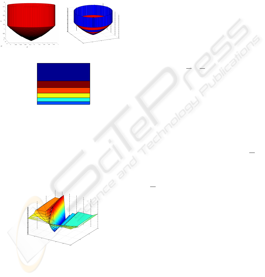
this parameterized convex shape can be approximated
with a set of parameterized linear inequalities and ob-
tain a double description of a parameterized polyhe-
dron as in figure 1b. A precutting in zones with reg-
ular shape (figure 1c) can help in the development of
explicit solution due to the important degree of redun-
dancy.
(a)
−1
−0.5
0
0.5
1
−1
−0.5
0
0.5
1
0
0.5
1
1.5
2
2.5
3
u1
u2
x2
(b)
−1 −0.8 −0.6 −0.4 −0.2 0 0.2 0.4 0.6 0.8 1
0
0.5
1
1.5
2
2.5
3
u1
u2
(c)
Figure 1: (a) The nonlinear dependence of the feasible do-
main on the parameters (b) The approximation by a param-
eterized polyhedron; (c) Regions in the parameters’ space
corresponding to redundancy-free constraints sets.
Finally the nonlinear MPC law for the system (15)
and the constraints (16) can be approximated by the
explicit solution found in terms of a piecewise linear
control law as in figure 2.
−6
−4
−2
0
2
4
6
0
2
4
6
−0.6
−0.4
−0.2
0
0.2
0.4
x
2
PWA function over 114 regions
x
1
f
Figure 2: Explicit solution as a piecewise linear function.
4.2 Nonconvex Feasible Domains
In the case when the convexity is lost, one can still
construct the convex hull (and an explicit solution)
associated with the non-convex domain. From the
resulting piecewise affine function one should retain
only those regions where the control law is feasible
w.r.t. the nonlinear constraints. For the violated con-
straints a distribution of points will be obtained. Fi-
nally the missing regions in the explicit solution will
be completed with the Voronoi partition correspond-
ing to these points on the concave border of the feasi-
ble domain.
Algorithm:
1. Obtain a set of points (
V ) on the frontier of the
feasible domain D (based on the nonlinear con-
straints).
2. Considering this set of points, construct the con-
vex
C
V
(which will include the non-convex do-
main D and some other infeasible domains from
the MPC point of view).
3. Split the set
V as V
L
∪
V
NL
∪
e
V ∪
b
V
•
b
V ∈ Int(C
V
)
•
e
V ∈ F(C
V
) and
C
V
=
C
V \
e
V
•
V
L
∈ F(
C
V
),
V
L
∩
e
V =
/
0 and V
L
saturate at
least one linear constraint in the MPC con-
straints;
•
V
NL
∈ F(
C
V
) and
V
NL
saturate no linear con-
straint
4.
C
V
is described in the dual representation by the
intersection of halfspaces
H (which represent the
faces of the convex hull C
V
). Split this set in
H ∪
b
H
•
b
H ⊂H such that ∃x ∈ C
V
with Sat(
b
H , x) 6=
/
0
and B(R
NL
,x) 6=
/
0
•
H = H \
b
H
5. Compute the unconstrained optimum k
∗
u
6. Project the unconstrained optimum on
C
V
:
k
∗
u
← Proj
C
V
{
−c
}
7. If k
∗
u
saturates a subset of constraints
K ⊂
b
H
(a) Retain the set of points:
S =
n
v ∈
b
V |∀x ∈C
V
s.t.Sat(
b
H , x) = K ;
B(R
NL
,x) = Sat(R
NL
,v)
}
(b) Construct the Voronoi partition for the colec-
tion of points in S
(c) Position k
∗
u
w.r.t. this partition and map the sub-
optimal solution k
∗
u
← v where v is the vertex
corresponding to the active region
EXPLICIT PREDICTIVE CONTROL LAWS - On the Geometry of Feasible Domains and the Presence of Nonlinearities
75
8. If the quality of the solution is not satisfactory,
improve the distribution of the points
V by aug-
menting the resolution around k
∗
u
and restart from
the step 2.
The following notations where used:
F(X) The frontier of a compact set X
Int(X) The interior of a compact set X
R
L
(D) The set of linear constraints in the defi-
nition of the feasible domain D
R
NL
(D) The set of nonlinear constraints in the
definition of the feasible domain D
Sat(R
∗
,x) The subset of constraints in R
∗
(ei-
ther R
L
either R
NL
) saturated by the vector x
B(R
∗
,x) The subset of constraints in R
∗
. vio-
lated by the vector x
4.2.1 Numerical Example
Consider the MPC problem implemented using the
first control action of the optimal sequence:
k
∗
u
= argmin
k
u
N
y
−1
∑
i=0
x
T
t+k
|
t
Qx
t+k
|
t
+ u
T
t+k
|
t
Ru
t+k
|
t
+
+x
T
t+N
y
|
t
Px
t+N
y
|
t
(17)
with
Q =
10 0
0 1
;R =
2 0
0 3
;P =
13.73 2.46
2.46 2.99
subject to
x
t+k+1
|
t
=
A
z
}| {
1 1
0 1
x
t+k
|
t
+
B
z
}| {
1 0
2 1
u
t+k
|
t
k > 0
−2
−2
6 u
t+k
|
t
6
2
2
0 6 k 6 N
y
−1
(u
1
t+k
|
t
)
2
+
u
2
t+k
|
t
−2
2
>
√
3 0 6 k 6 N
y
−1
(u
1
t+k
|
t
)
2
+
u
2
t+k
|
t
+ 2
2
>
√
3 0 6 k 6 N
y
−1
u
t+k
|
t
=
0.59 0.76
- 0.42 - 0.16
| {z }
K
LQR
x
t+k
|
t
N
u
6 k 6 N
y
−1
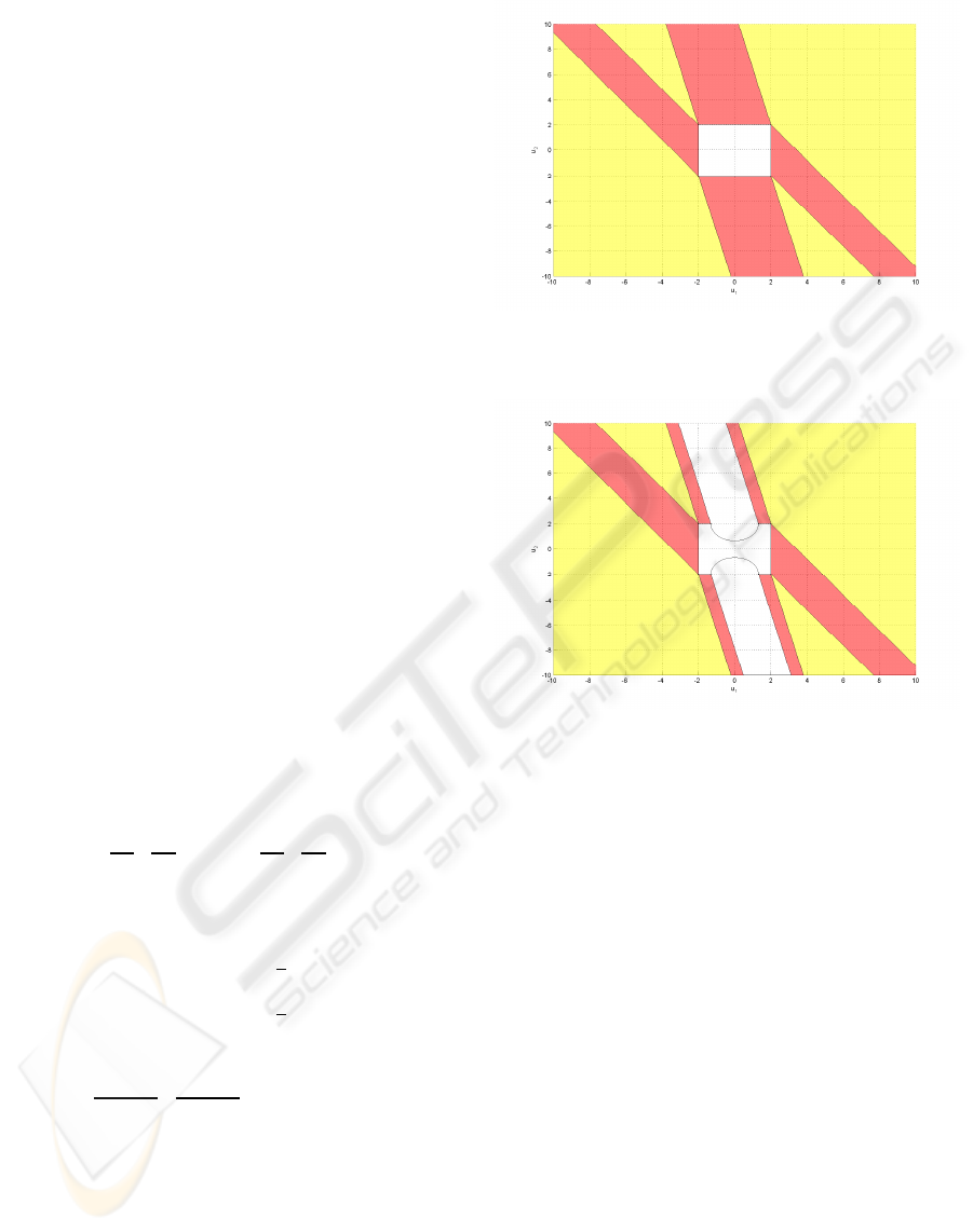
One can observe the presence of both linear and
nonlinear constraints. By following the previous al-
gorithm, in the first stage, the partition of the state
space is performed by considering only the linear con-
straints (figure 3).
Each such region correspond with a specific pro-
jection law. By simply verifying the regions where
this projection law obey the nonlinear constraints, the
exact part of the explicit solution is obtained (fig. 4).
Figure 3: Partition of the arguments space (linear con-
straints only).
Figure 4: Retention of the regions with feasible linear pro-
jections.
Further, a distribution of points on the nonlinear
frontier of the feasible domain has to be obtained
and based on this distribution of points the associated
Voronoi partition constructed. By superposing it to
the regions not covered (white zones in the figure 4)
at the previous step, one obtain a complete covering
of the arguments space. Figure 5 depicts such a com-
plete partition for distribution of 10 points for each
nonlinear constraint.
By correspondence, the figure 6 describes the par-
tition of the state space for the explicit solution.
Finally the complete explicit solution is depicted
in figure 7. The discontinuities are observable in the
regions generated upon the Voronoi partition. In or-
der to give an image of the complexity it can men-
tioned that the explicit solutions contains 31 regions
the computational effort was less than 2s mainly spent
in the construction of the Voronoi partition.
ICINCO 2007 - International Conference on Informatics in Control, Automation and Robotics
76
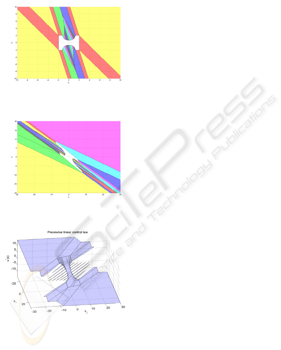
Figure 5: Partition of the arguments space (nonlinear case)
- 10 points per nonlinear constraint.
Figure 6: Partition of the state space - 10 points per nonlin-
ear constraint.
Figure 7: Explicit control law - 10 points per nonlinear con-
straint.
5 CONCLUSION
The parameterized polyhedra offer a transparent char-
acterization of the MPC degrees of freedom. Once
the complete description of the feasible domain as a
parameterized polyhedron is obtained explicit MPC
laws can be constructed using the projection of the
unconstrained optimum. The topology of the feasible
domain can lead to explicit solution even if nonlinear
constraints are taken into consideration. The price to
be paid is found in the degree of suboptimality.
REFERENCES
Bemporad, A., Borrelli, F., and Morari, M. (2001). Robust
Model Predictive Control: Piecewise Linear Explicit
Solution. In European Control Conference, pages
939–944, Porto, Portugal.
Bemporad, A., Morari, M., Dua, V., and Pistikopoulos, E.
(2002). The Explicit Linear Quadratic Regulator for
Constrained Systems. Automatica, 38(1):3–20.
Borelli, F. (2003). Constrained Optimal Control of Linear
and Hybrid Systems. Springer-Verlag, Berlin.
Goodwin, G., Seron, M., and Dona, J. D. (2004). Con-
strained Control and Estimation. Springer, Berlin.
Kerrigan, E. and Maciejowski, J. (2004). Feedback min-
max model predictive control using a single linear pro-
gram: Robust stability and the explicit solution. In-
ternational Journal of Robust and Nonlinear Control,
14(4):395–413.
Leverge, H. (1994). A note on chernikova’s algorithm. In
Technical Report 635. IRISA, France.
Loechner, V. and Wilde, D. K. (1997). Parameterized poly-
hedra and their vertices. International Journal of Par-
allel Programming, V25(6):525–549.
Motzkin, T.S., R. H. T. G. and R.M., T. (1953). The Dou-
ble Description Method, republished in Theodore S.
Motzkin: Selected Papers, (1983). Birkhauser.
Olaru, S. and Dumur, D. (2005). Compact explicit mpc with
guarantee of feasibility for tracking. In 44th IEEE
Conference on Decision and Control, and European
Control Conference. CDC-ECC ’05., pages 969–974.
Olaru, S. B. and Dumur, D. A parameterized polyhedra
approach for explicit constrained predictive control.
In 43rd IEEE Conference on Decision and Control,
2004. CDC., pages 1580–1585 Vol.2.
Schrijver, A. (1986). Theory of Linear and Integer Pro-
gramming. John Wiley and Sons, NY.
Scokaert, P. O., Mayne, D. Q., and Rawlings, J. B. (1999).
Suboptimal model predictive control (feasibility im-
plies stability). In IEEE Transactions on Automatic
Control, volume 44, pages 648–654.
Seron, M., Goodwin, G., and Dona, J. D. (2003). Charac-
terisation of receding horizon control for constrained
linear systems. In Asian Journal of Control, volume 5,
pages 271–286.
Tondel, P., Johansen, T., and Bemporad, A. (2003). Evalua-
tion of piecewise affine control via binary search tree.
Automatica, 39:945–950.
Wilde, D. (1993). A library for doing polyhedral operations.
In Technical report 785. IRISA, France.
EXPLICIT PREDICTIVE CONTROL LAWS - On the Geometry of Feasible Domains and the Presence of Nonlinearities
77
