
MULTIPLE-MODEL DEAD-BEAT CONTROLLER IN CASE OF
CONTROL SIGNAL CONSTRAINTS
Emil Garipov, Teodor Stoilkov
Technical University of Sofia, 1000 Sofia, Bulgaria
Ivan Kalaykov
¨
Orebro University, 70182
¨
Orebro, Sweden
Keywords:
Dead-beat controller, multiple-model control, single-input single-output systems.
Abstract:
The task of achieving a dead-beat control by a linear DB controller under control constraints is presented in
this paper. Two algorithms using the concept of multiple-model systems are proposed and demonstrated - a
multiple-model dead-beat (MMDB) controller with varying order using one sampling period and a MMDB
controller with fixed order using several sampling periods. The advantages and disadvantages of these con-
trollers are summarized.
1 INTRODUCTION
The Dead-Beat (DB) control problem in discrete time
control theory consists of finding an input signal,
which provides a transient response in a minimum
number of sampling time steps. It has been studied by
many researchers, e.g. (Jury, 1958), (Kucera, 1980),
(Kaczorek, 1980), (Isermann, 1981), etc. If an n
th
or-
der linear system is null controllable, this minimum
number of steps is n, as the applied feedback provides
all poles of the closed-loop transfer function at the
z-plane origin. The linear case is easy to solve, but
DB control for non-linear systems is an open research
problem (Nesic et al., 1998).
The DB controller of normal order (Isermann,
1981), denoted as DB(n,d), provides a constant con-
trol action after n
s
= (n+ d) sampling steps, where d
is the plant delay. For small sampling period the lin-
ear DB(n,d) controller forms extremely high control
values at the first and second sampling steps after a
step change of the system reference signal. In gen-
eral, the control valve constrains the control signal, so
these high amplitudes cannot be passed to the plant,
thus making the system to be non-linear.
One way to solve the problem of constrained con-
trol signal, and still keeping the system as linear, is to
prolong the transient response by increasing the con-
troller order n
s
. Isermann (1981) suggested increased
by one order DB(n,d,1) controller, so the transient re-
sponse takes n
s
= (n+ d+1) sampling steps with de-
creased control value compared to the DB(n,d). This
approach did not have essential practical application,
but suggested two ideas:
- a higher controller order reduces the maximal
amplitude of the control action;
- linear dead-beat control can be achieved by flex-
ible tuning of the controller numerator coefficients.
In (Garipov and Kalaykov, 1991) an approach for
design of adaptive DB(n,d,m) controller is presented,
where the order increment m is sequentially changed
until the control signal fits the control constraints. The
reduction of the control magnitude pays off the pro-
longation of the transient response, as the signal en-
ergy distributes in more sampling time steps. Another
approach is to increase the system sampling period
without losing information. A control system with
two sampling periods is proposed in (Garipov and
Stoilkov, 2004) as a compromise solution.
These last two above mentioned approaches are
useful for generalizing them by merging and involv-
ing various aspects of the multiple-model concept, as
presented in (Murray-Smith and Johansen, 1997). In
the present paper the task is solved by multiple-model
dead-beat controller (MMDB) for one fixed and sev-
eral sampling periods of the control system.
In Section 2 we present the theoretical base for
design of DB controller of increased order. In Sec-
tion 3 we describe the operation principle of DB con-
trol based on two sampling periods. In Section 4 the
MMDB controller concept is developed in two vari-
ants. The first is based on a set of DB controllers of
increased order in a system with one sampling period.
171
Garipov E., Stoilkov T. and Kalaykov I. (2007).
MULTIPLE-MODEL DEAD-BEAT CONTROLLER IN CASE OF CONTROL SIGNAL CONSTRAINTS.
In Proceedings of the Fourth International Conference on Informatics in Control, Automation and Robotics, pages 171-177
DOI: 10.5220/0001633901710177
Copyright
c
SciTePress

The second is utilizing a set of normal order DB con-
trollers designed for several sampling periods. The
concluding section summarizes the main properties of
the proposed DB controllers.
2 DESIGN OF DB CONTROLLER
OF INCREASED ORDER
Let the control plant description be:
W
o
(z) =
B(z)
A(z)
z
−d
=
=
b
1
z
−1
+ b
2
z
−2
+ ... +b
n
z
−n
1+ a
1
z
−1
+ a
2
z
−2
+ ... + a
n
z
−n
z
−d
(1)
According (Garipov and Kalaykov, 1991) the de-
signed DB(n,d,m) controller is
W
p
(z) =
Q(z)
1− z
−d
P(z)
=
=
q
0
+ q
1
z
−1
+ ... + q
n+m
z
−(n+m)
1− z
−d
(p
1
z
−1
+ p
2
z
−2
+ ... + p
n+m
z
−(n+m)
)
(2)
The vector θ of (2n+2m+1) unknown coefficients
of the DB controller can be determined from the fol-
lowing matrix equation
X θ = Y, (3)
X =
X
∗
··· ··· ···
D
z
.
.
. Z
, Y =
Y
∗
···
D
y
, θ =
p
(1)
p
(2)
q
(1)
q
(2)
,
X
∗
=
E
1
.
.
. D
e
··· · ·· ···
.
.
. ··· · · · ···
A
1
.
.
. −B
1
··· · ·· ···
.
.
. ··· · · · ···
D
a
.
.
. A
2
.
.
. D
b
.
.
. −B
2
,
dimX
∗
= (2n+ m+ 1) × (2n+ 2m+ 1),
Y
∗
=
1
0
.
0
, p
(1)
=
p
1
p
2
.
p
m
, p
(2)
=
p
1+m
p
2+m
.
p
n+m
,
q
(1)
=
q
0
q
1
.
q
m
, q
(2)
=
q
1+m
q
2+m
.
q
n+m
.
dimY
∗
= (2n+ m+ 1) × 1,
A
1
=
a
0
0 . . . . 0
a
1
a
0
0 . . . 0
. . . . . . .
. . . . . . .
a
n
a
n−1
. a
0
0 . 0
0 a
n
. . a
0
. 0
. . . . . . .
. . . . . . .
0 0 . a
n
a
n−1
. a
0
,
dimA
1
=(n+m)× (n+m),
B
1
=
b
1
0 . . . . 0 0
b
2
b
1
0 . . . 0 0
. . . . . . . .
b
n
b
n−1
. b
1
. . 0 0
0 b
n
. . b
1
0 . 0
. . . . . . . .
. . . . . . . .
. . . . . . . .
0 . 0 b
n
. . b
1
0
,
dimB
1
=(n+m)× (n+m+1),
A
2
=
a
n
a
n−1
. a
1
0 a
n
a
n−1
a
2
. . . .
0 0 . a
n
,
B
2
=
b
n
b
n−1
. b
1
0 b
n
. b
2
0 0 . .
0 0 . b
n
dimA
2
= n× n, dimB
2
= n× n,
E
1
=[ 1 1 1 . . . 1],
D
e
, D
a
, D
z
, D
y
are matrices with zero elements,
dimD
e
= 1×(n+ m+ 1) , dimD
a
= n×m, dimD
b
=
n× (m+ 1) , dimD
z
= m× (n+ m), dimD
y
= m× 1.
The only solution of (3), which is the goal of
dead-beat controller design task, is achieved when the
rank of the linear system (3) is full. In fact this de-
pends on the initially undetermined block matrix Z,
dimZ = m× (n+m+ 1). The z
ij
values can be chosen
in accordance with intention of the designer to guar-
antee desired control u(k) such that additional m be-
havior conditions based on the following dependen-
cies between parameters and signals:
a) When step change of the reference signal takes
place at the k
th
sampling step, the DB controller nor-
mally produces the largest positive amplitude u(k) at
k
th
sampling step, followed by a smaller and negative
value u(k+1) at (k+1)
th
sampling step. Therefore, if
the signal energy after the k
th
sampling step is dis-
tributed over two or more sampling steps, holding the
control signal, the large control magnitudes will be
reduced (Isermann, 1981). This can be described by
the inequality
ICINCO 2007 - International Conference on Informatics in Control, Automation and Robotics
172

Mod
{
u(k+ i)
}
|
u(k+i+1)=u(k+i)
<
Mod
{
u(k+ i)
}
|
u(k+i+1)6=u(k+i)
i = 0, 1, ..., which should be related to the initially de-
termined physical constraints on the control u(k).
b) The matrix Z is needed only for dead-beat con-
trollers of increased order, i.e. only when m > 1.
Each row of it consists of one additional simple condi-
tion based on Isermann’s idea for holding the previous
value of the control signal
u(k+ i+ 1) = u(k + i), i = 0, 1, ..., (4)
for certain number of time steps. According (Garipov
and Kalaykov, 1991), such behavior can be obtained
by properly setting the coefficients of the polyno-
mial Q(z) of (n + m)
th
order. As always q
0
6= 0 and
q
n+m
6= 0, if we set q
i+1
= 0 we obtain the desired
condition u(k + i + 1) = u(k+ i). Therefore the val-
ues z
ij
play a special role of pointing which coefficient
q
i+1
is selected to be zero. When all values z
ij
=0, it is
assumed all coefficients q
i+1
are nonzero. Therefore,
first we have to zero the matrix Z and then set one unit
value in the rows of Z. More details for how to select
the values are given in (Garipov and Kalaykov, 1991).
c) If we want to hold the control signal longer time
according condition (4), we have to zero more neigh-
bor coefficients in Q(z) by manipulating two or more
neighbor rows of Z.
As an illustrative example let us take a plant with
a continuous transfer function
W
o
(s) =
2s+ 1
(10s+ 1)(7s+ 1)(3s+ 1)
e
−4s
For a sampling period T
o
= 4 sec. we get
W
o
(z) =
0.06525z
−1
+ 0.04793z
−2
− 0.00750z
−3
1− 1.49863z
−1
+ 0.70409z
−2
− 0.09978z
−3
z
−1
,
n
a
= n
b
= n = 3, d = 1
Three dead-beat controllers with different struc-
tures: DB(3,1,0), DB(3,1,1) – three variants and
DB(3,1,2) – six variants are designed according to
the approach (Garipov and Kalaykov, 1991). It these
variants some of the Q(z) coefficients were zeroed.
Obviously, the bigger is m the more variants of ze-
roing exist. Table 1 represents the maximum and
minimum control values of the control signal during
the transient response. The normal order DB con-
troller (m=0) provides the largest values, while vari-
ant1 when m = 1 and m = 2 provide significantly
smaller values, which could fit to the control signal
constraints.
Table 1: Max and min control values for the example.
m Variant # u
max
u
min
0 9.46 -4.71
1 variant1 3.78 -2.05
1 variant2 6.43 -0.18
1 variant3 8.28 -2.95
2 variant1 2.34 -0.83
2 variant2 3.01 0.28
2 variant3 3.49 -0.14
2 variant4 5.13 0.62
2 variant5 5.94 0.12
2 variant6 5.94 -2.27
3 DEAD-BEAT CONTROLLER IN
A SYSTEM WITH TWO
DIFFERENT SAMPLING
PERIODS
The concept of DB controller of increased order, as
described in the previous section, is one way of hold-
ing the control signal during more sampling steps of
the transient response and consequently redistributing
the signal energy in time. In this section we present an
alternative approach employing nearly the same idea
for redistributing the signal energy in time. To pro-
long the transient response and still keep the system
null controllable, we can increase the sampling period
for which we design a DB controller of normal or-
der DB(n,d,0), but implement this controller in a sys-
tem operating at smaller sampling rate. The concept
(Garipov and Stoilkov, 2004) can be demonstrated by
the discrete-continuous control system with two dif-
ferent sampling periods as shown on Fig.1. In fact
this is a kind of internal model control (IMC) scheme,
the inner loop of which is designed for a large sam-
pling interval, and the outer loop is operating a small
sampling interval. The main idea is that the main con-
troller should work at the large sampling interval, thus
redistributing the control signal energy in time and
providing smaller control signal magnitude. But at the
same time the entire system should operate at smaller
sampling interval, therefore a correction signal from
the plant-model difference should close the system.
The “Discrete Controller” block provides the con-
trol u to the “Continuous Plant” block (assumed to be
linear with known time delay). Two different sam-
pling periods are introduced:
• small sampling period T
CS
0
, which is fundamental
for the entire system, meaning that all signals are
sampled and propagate at this period;
• large sampling period T
Reg
0
= l.T
CS
0
, l > 1,used
MULTIPLE-MODEL DEAD-BEAT CONTROLLER IN CASE OF CONTROL SIGNAL CONSTRAINTS
173
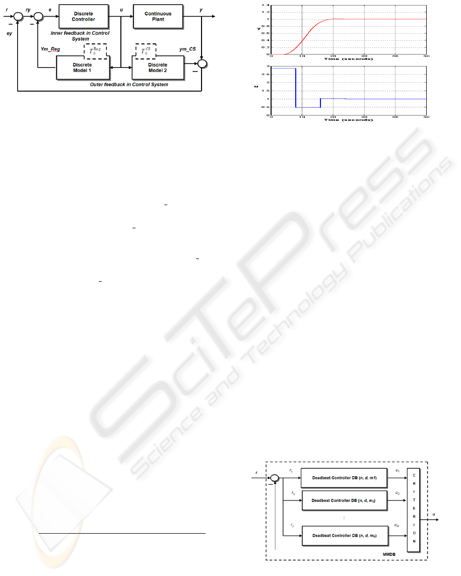
Figure 1: Discrete-continuous control system operating
with two different sampling periods.
to define “Discrete Model 1” and respectively in
the design of the “Discrete Controller” block.
In fact, the system contains two feedback loops:
• outer loop, which forms corrected reference sig-
nal ry = r – ey by the error ey = y – ym
CS between
the measured output y of the “Continuous Plant”
and the calculated output ym CS of the “Discrete
Model 2”;
• inner loop, forming the error e = ry – ym Reg
in the system between corrected reference ry and
calculated output ym
Reg of “Discrete Model 1”.
As an illustrative example let us take the same sys-
tem given in Section 2. If we select a small sam-
pling period T
o
=0.1 sec, the normal order DB(n,d,0)
controller produces extremely high control signal am-
plitude u(0) = 216130 after the unit step change of
the reference signal. Obviously this value will be
“clipped” by the control valve and the system perfor-
mance will deteriorate. We decide to keep T
CS
0
= 0.1
sec as a fundamental sampling period for the entire
system, but introduce a second large sampling pe-
riod T
Reg
0
= 8 sec for which a DB controller is de-
signed. Even T
Reg
0
= 8 sec does not seem to be
good choice, we intentionally use here for illustra-
tion. Hence, in the inner loop we have to use the “Dis-
crete Model1”, which is sampled at T
Reg
0
= 8 sec, for
providing proper control signal behavior. The outer
loop is to correct the reference signal depending on
the “Discrete Model2” operating at T
CS
0
= 0.1 sec
(nearly continuous-time control). The designed DB
Controller for T
Reg
0
=8 sec is:
W
o
(z) =
2.8653− 2.4004z
−1
+ 0.5635−2− 0.0285z
−3
1− 0.6045z
−1
− 0.3991z
−2
+ 0.0036z
−3
,
The first numerator coefficient q
o
=2.8653 is equal
theoretically to the control value u(0). Fig. 2
demonstrates the controlled output (top) and the con-
trol signal (bottom), which has acceptable amplitude
u(0)=2.8653 exactly as expected. The finite transient
response takes 24 sec that is exactly three times T
Reg
0
,
as the system is of third order.
Figure 2: System with sampling period T
CS.
0
= 0, 1 sec and
DB controller, designed for T
Reg
0
= 8 sec.
4 MULTIPLE-MODEL
DEADBEAT CONTROLLER
4.1 MMDB Controller with Varying
Order using One Sampling Period
The existence of control signal constraints by the con-
trol valve clearly indicates the needs to guarantee a
control magnitude that always fits within the control
constraints for all operating regime of the system.
The closer is the operating point to the constraints
the bigger should be the DB controller order, as al-
ready clarified in Section 2. Obviously increasing the
order the transient response becomes longer, but it
is more important to keep the control signal within
the constraints paying with the longer finite time of
the response. As the plant operating point continu-
ously changes, we should select the minimal order of
the DB controller that satisfies the control signal con-
straints. So we came to the idea of building a MMDB
controller that combines several DB controllers of dif-
ferent order running in parallel. The MMDB consists
of two major parts:
Figure 3: Structure of the MMDB.
- a set of N DB(n,d,m) controllers for the given model
of the controlled plant, each of which is designed for
different values of m, namely m
1
, m
2
, ... , m
N
, such
that all they provide constrained control signal within
ICINCO 2007 - International Conference on Informatics in Control, Automation and Robotics
174
the constraints of the control valve [u
min
, u
max
]for all
possible variations of the reference signal; one sam-
pling interval is assumed;
- a “criterion” block that switches the input of the
plant to the output of one of the DB(n,d,m) controllers
depending on a predefined set of conditions, in this
case checking the output of which of the DB(n.d,m)
controllers is within the constraints [u
min
, u
max
]. Ad-
ditional criterion is to select the individual DB con-
troller having the minimal value of m
i
, because then
the transient response is of minimum duration. As
Figure 4: Reference signal and plant output (top); control
signal within the constraints (middle); increment of the DB
controller order (bottom).
an example we designed a MMDB controller for the
plant described in Section 2 with sampling period
T
Reg
0
= 4sec. A set of DB controllers is included,
namely DB(3,1,m), m = 0, 1, 2, 3, 4 and 5. On Fig.
4 the transient response of the plant follows the ref-
erence signal, but is stepwise as the sampling period
is big. The control signal lies within the constraints.
The “criterion” block decides to switch the appropri-
ate DB(n,d,m
j
) controller such that the constraints are
satisfied, as seen on the bottom picture on Fig. 4.
The “criterion” block is selecting an individual con-
troller with higher or smaller order depending on the
distance of the plant operating regime to the control
constraints and the step change magnitude of the ref-
erence.
The important property of the proposed MMDB
controller is the embedded flexibility to select the ap-
propriate order of the DB controller. For compari-
son on Fig. 5 we present the performance of fixed
DB(3,1,0) and DB(3,1,1) controllers at the same op-
erating conditions. Obviously the transient response
does not represent a deadbeat behavior as a result of
applying too low DB controller order, which cannot
bring the control signal within the constraints.
Figure 5: Plant output and reference signal for DB(3,1,0)
(top) and DB(3,1,1) (bottom) controller.
4.2 MMDB Controller with Fixed
Order using Several Sampling
Periods
Contrary to the concept presented in Section 4, here
we suggest a MMDB controller that contains a num-
ber of controllers, each of which is designed for dif-
ferent sampling periods T
Reg
i
0
, i=1, 2, ..., N, assum-
ing that the entire control system operates with a sam-
pling period T
CS
0
<< T
Reg
i
0
, as shown on Fig. 6.
The difference between this MMDB and the
MMDB on Fig. 3 is the content of the individual DB
controllers. Here they are assumed of DB(n,d,0) type
(normal order DB controller), but they differ due to
the different sampling period used for their design.
Generally, there is no limitation to use DB(n,d,m)
type controllers as well, but for simplicity m is not
considered to be a parameter of choice. As an exam-
Figure 6: Structure of the MMDB.
ple we demonstrate a MMDB controller for the plant
described in Section 2 with sampling period T
CS
0
= 0.1
sec. A set of DB controllers is designed for T
REG
0
=
4, 6, 8, 10, 12, 14 and 18 sec. The performance of
the system is shown on Fig. 7. One can see that the
transient response of the plant follows the reference
signal and is rather smooth due to the small sampling
period of the entire system. The control signal lies
within the constraints. On the bottom picture on Fig.
MULTIPLE-MODEL DEAD-BEAT CONTROLLER IN CASE OF CONTROL SIGNAL CONSTRAINTS
175
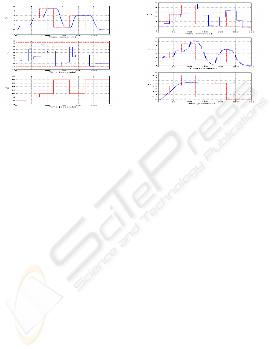
Figure 7: Reference signal and plant output (top); control
signal within the constraints (middle); sampling period of
the DB controller (bottom).
7 it can be seen that the “criterion” block is selecting
an individual controller designed for bigger higher or
smaller sampling period depending on the distance of
the plant operating regime to the control constraints
and the magnitude of the step change of the reference
signal.
The important property of the proposed MMDB
controller with fixed order is the possibility to se-
lect the appropriate sampling period of the DB con-
troller that keeps the control signal within the con-
straints. For comparison on Fig. 8 we present the per-
formance of fixed DB(3,1,0) controller designed and
implemented at the same sampling period T
Reg
0
= T
CS
0
and the same operating conditions. Obviously the
transient response does not represent a deadbeat be-
havior as a result of applying too low DB controller
order, which cannot bring the control signal within
the constraints.
5 CONCLUSION
Two original ideas for solving the task of achieving a
dead-beat control by a linear DB controller under con-
trol constraints were presented in this paper: for de-
sign of DB controllers of increased order and for im-
plementation of a discrete-continuous control system,
which operates with two different sampling periods.
Two algorithms using the concept of multiple-model
systems were proposed and demonstrated – a MMDB
controller with varying order using one sampling pe-
riod and a MMDB controller with fixed order using
several sampling periods. Both algorithms provide
normal operating of the control system and control
signal does not leave the predefined constrains. Nu-
Figure 8: Plant output and reference signal for: T
Reg
0
=
T
CS
0
=18 sec (top); T
Reg
0
= T
CS
0
=4 sec (middle); T
Reg
0
=
T
CS
0
= 0.1 sec (bottom).
merical simulations confirm the performance of the
proposed algorithms.
The advantages and disadvantages of these con-
trollers are summarized in Table 2, which can be a
useful tool for selection of DB controllers in practical
applications.
ACKNOWLEDGEMENTS
The third author acknowledges the support of the
Swedish KKS Foundation for part of this research.
REFERENCES
Garipov, E. and Kalaykov, I. (1991). Design of a class ro-
bust self-tuning controllers. In Prepr. of IFAC Symp.
on Design Methods.
Garipov, E. and Stoilkov, T. (2004). Multiple-model dead-
beat controller in control systems with variable sam-
pling period. In Annual Proc. of the Technical Univer-
sity Sofia.
Isermann, R. (1981). Digital Control Systems. Springer
Verlag, Berlin.
Jury, E. (1958). Sampled-Data Control Systems. Wiley,
New York.
Kaczorek, T. (1980). Deadbeat control of single-input
single-output linear time-invariant systems. Int. J.
Syst. Sci., 11:411–421.
Kucera, V. (1980). A dead-beat servo problem. Interna-
tional Journal of Control, 32:107–113.
Murray-Smith, R. and Johansen, T. A. (1997). Multiple
Model Approaches to Modeling and Control. Taylor
and Francis, London.
Nesic, D., Mareels, M., Bastin, G., and Mahony, R. (1998).
Output dead beat control for a class of planar polyno-
mial systems. SIAM J. Control Optim., 36:253–272.
ICINCO 2007 - International Conference on Informatics in Control, Automation and Robotics
176

Table 2: Basic properties of the Dead-beat controllers.
Controller Advantages Disadvantages
• DB controller of
normal order,
system with one
model and one
sampling period
• Easy tuning of the controller with small
design efforts.
• Large control amplitudes for models of low
order and small time delays for small sam-
pling period.
• Rough response to the reference signal
when big sampling period is used.
• No adaptive properties when changing the
operating regimes of the control system.
• DB controller of
increased order,
system with one
model and one
sampling period
• Possibility of multi variant tuning.
• Good control and significant reduction
of the large control amplitudes at the first
few sampling steps.
• Smoother response even for small sam-
pling period, due to the increased con-
troller order.
• Relatively complex design algorithm.
• Higher order of the controller needed to re-
duce the large control amplitudes.
• No adaptive properties when changing the
operating regimes of the control system.
• DB controller of
normal order,
system with
one model and
two different
sampling periods
• Simple controller design algorithm.
• Good control and significant reduction
of the large control amplitudes at the first
few sampling steps.
• Smoother response to the reference sig-
nal even for small sampling period, due
to the increased controller order.
• Complicated scheme of the control system.
• No adaptive properties when changing the
operating regimes of the control system.
• MMDB con-
troller using
increased order
DB blocks,
system with one
sampling period
• Adaptation to changes in operating
regimes of the control system in case of
complex profile of the reference signal
and controller output constraints.
• Good control and significant reduction
of the large control amplitudes at the first
few sampling steps.
• Smoother response even for small sam-
pling period, due to the increased con-
troller order.
• Relatively complex design algorithm.
• Complicated scheme of the control sys-
tem, as several DB controllers with differ-
ent fixed structures but with one sampling
period function at different operating points
of the control system.
• Need of supervisor for switching between
various controllers.
• MMDB con-
troller using
normal order DB
blocks,
system with sev-
eral sampling pe-
riods
• Adaptation to changes in operating
regimes of the control system in case of
complex profile of the reference signal
and controller output constraints.
• Good control and significant reduction
of the large control amplitudes at the first
few sampling steps.
• Smoother response even for small sam-
pling period, due to the increased con-
troller order.
• Simple algorithm for designing DB con-
troller of normal order.
• Complicated scheme of the control sys-
tem, as several DB controllers with differ-
ent fixed structures but with one sampling
period function at different operating points
of the control system.
• Need of supervisor for switching between
various controllers.
MULTIPLE-MODEL DEAD-BEAT CONTROLLER IN CASE OF CONTROL SIGNAL CONSTRAINTS
177
