Ultrasound Sensor Array for Robust Location
Jos
´
e N. Vieira
1
, S
´
ergio I. Lopes
2
, Carlos A. C. Bastos
1
and Pedro N. Fonseca
1
1
Departamento de Electr
´
onica, Telecomunicac¸
˜
oes e Inform
´
atica / IEETA
Universidade de Aveiro 3810-193 Aveiro, Portugal
Abstract. In this paper we present a system for localizing a team of soccer robots
using ultrasound. The proposed system uses chirp signals to obtain a better signal
to noise ratio with good time resolution and improved interference immunity.
An array of four ultrasonic sensors is used to obtain spatial diversity and reduce
the localization error. An efficient DSP algorithm for base-band conversion and
decimation of the received pulses is also presented. The proposed system based
on the TI DSP 2812 is very efficient and allows the localization of the robots up
to 8 meters with an angular error with a maximum standard deviation of 2°.
1 Introduction
Ultrasonic Sensors (USS) systems are widely used in robotics for obstacle localization
and mutual robot localization [1], [2]. Most of the commercial available ultrasonic sys-
tems use a sinusoidal pulse to measure the Time of Flight (TOF). Usually these systems
perform badly in the presence of interferences and various authors have presented more
complex alternatives using different types of modulation of the emitted ultrasonic pulse
[3] and [4].
This paper describes an ongoing work to build a localization system, using USS
for a team of soccer robots. The main achievements of this work are the efficient im-
plementation of the baseband converter of the received bandpass chirp pulses, and the
array with four sensors using an algorithm that integrates several measurements in time
and space resulting in a small error for distances up to 8 meters.
The specifications for this system require that it should be able to locate each of
the mobile robots (MR) with an accuracy better than ±0.5 meters for distances up to 8
meters.
Since the goalkeeper has reduced mobility and its position can easily be determined
by the vision location system, all the positions of the other robots are referenced to its
position. The goalkeeper has an array of four aligned sensors at 20cm from each other
as can be seen in figure 1. Each field MR has four emitters and receivers equally spaced
over a circle and working like a transponder. The measurement of the position of each
MR is performed in the following way: the goalkeepere emits an ultrasound start signal,
then each MR answer after n×50ms where n is the MR number ID. This guarantees the
time interleaving of the answers. The goalkeeper evaluates the distance to each robot n
by
d
n
= c(T
n
− n × 50ms) = cT OF
n
, (1)
N. Vieira J., I. Lopes S., A. C. Bastos C. and N. Fonseca P. (2007).
Ultrasound Sensor Array for Robust Location.
In Proceedings of the 3rd International Workshop on Multi-Agent Robotic Systems, pages 84-93
Copyright
c
 SciTePress

where T is the total measured time between the start signal and the received signal
from the MR, T OF is the time of flight and c the sound speed.
2 Localization System
A previous version of the localization system had only two receivers located 20cm
apart. This system was very sensible to small errors in the TOF measurements leading
to an unusable system [5]. We solved this problem by acting on various aspects of the
system. Firstly, we increased the applied voltage to the transmitter from 8 to 16Volts.
Then we built an array with four aligned sensors spaced 20cm from each other to obtain
spatial diversity and as a consequence increased stability in position evaluation. Finally,
we improved the algorithm that evaluates the (x
m
, y
m
) by integrating several sets of
four measures T
i
to get an extra gain in the position stability.
The digital signal processing of the localization system is carried out by a DSP2812.
If all the digital signal processing was performed at the sampling frequency of 160kHz,
the DSP 2812 would not have enough processing power to calculate the TOF for the four
channels. In order to circumvent this limitation, we implemented a baseband converter
that outputs the decimated quadrature and phase components of the input signal. The
baseband converter was implemented directly in DSP2812 assembly language and it
uses about 50% of the available DSP processing power. The baseband converter reduces
the sampling frequency by a factor of 32, from 160kHz to 5kHz. The processing of the
converter output is much less demanding on the processing power and was implemented
in C.
2.1 Time of Flight Measurement
The transmitted chirp pulse is generated by sampling the signal
c(t) = h(t) cos

ω
1
t + βt
2

, t ∈ [0 . . . T ] ,
with β = (ω
2
− ω
1
)/(2T ), where ω
1
and ω
2
are the initial and final frequencies of
the chirp, T is the duration of the pulse and h(t) is a Hamming window. The window
h(t) is used to reduce the side lobes that appear on the autocorrelation of the chirp. The
carrier frequency is defined as ω
c
= (ω
1
+ ω
2
)/2.
Figure 2 shows the chirp autocorrelation with and without the Hamming window.
The reduction of the sidelobes is important to avoid false peak detection.
Baseband converter For bandpass signals, the Nyquist theorem states that a signal
has to be sampled at a frequency not less than twice the bandwidth of the signal. Since
the bandwidth of c(t) is typically 2kHz (in our system) it is possible to reduce the
sampling frequency to a much lower value (5kHz) by performing a bandpass to lowpass
transformation (see figure 3). This technique is well known and widely used on radar
and ultrasound sensing [6]. Several methods are available to perform this conversion
e.g. [7].

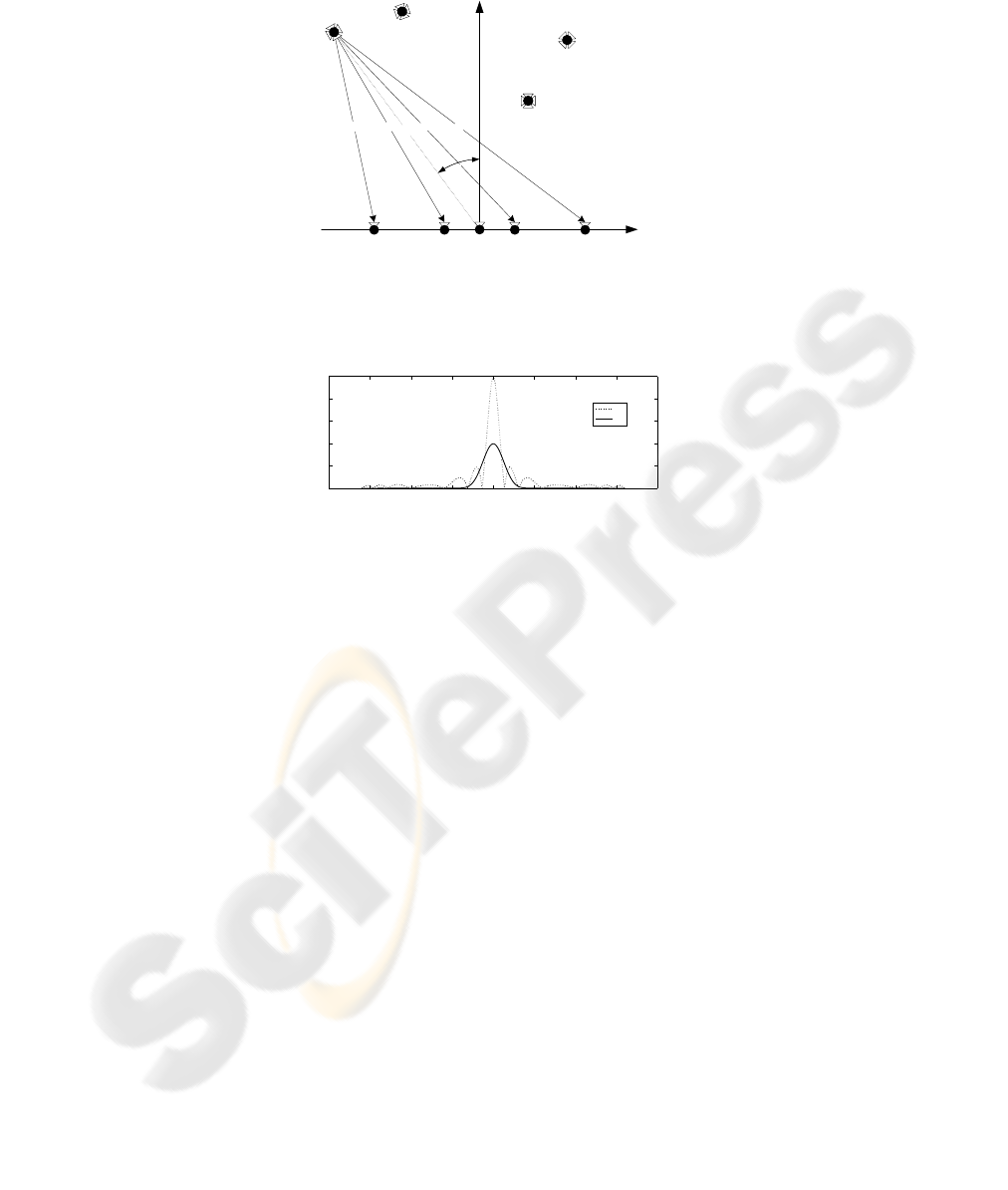
d
3
d
0
d
1
d
2
USS
0
(-0.3,0)
USS
1
(-0.1,0)
(0,0)
USS
2
(0.1,0)
USS
3
(0.3,0)
MR
0
(x
m
,y
m
)
d
m
θ
x [m]
y [m]
MR
1
MR
2
MR
3
Fig.1. Locating the MR with the four sensor USS
i
array and the goalkeeper emitter (located at
the origin).
−8 −6 −4 −2 0 2 4 6 8
0
0.2
0.4
0.6
0.8
1
ms
R
cc
R
cw
Fig.2. Cross correlation of the chirp (dotted line) and the chirp multiplied by a Hamming window
(solid line).
In this system we used low cost ultrasonic transducers from Murata that have a large
aperture (MA40S4R and MA40S4S), essential to cover all the field. Their bandpass
frequency response is centered at 40kHz with a useful bandwidth of 2kHz. The emitted
pulses are chirps ranging from 39 to 41kHz with a duration of 6.4ms. As the baseband
converted chirp has a bandwidth of only 1kHz the signal is decimated by 32 resulting
in a sampling frequency of 5kHz which is enough to represent the signal.
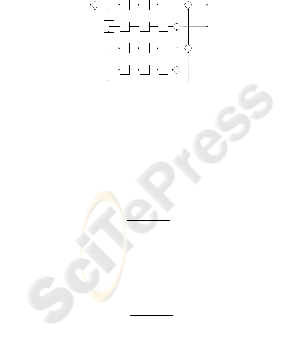
Figure 4 shows the structured of the baseband converter as implemented in this
work. We managed to simplify the calculations needed to perform the baseband con-
version by specifying an integer relation between the sampling frequency and the carrier
frequency and by integrating the modulators within the filters structure. The filter was
implemented using a polyphase decomposition [8]. In order to calculate both outputs
x
i
and x
q
, the system only has to perform N/D product-accumulation operations for
each input signal sample, where N is the number of coefficients of the filter and D the
decimation factor. As the filter H(z) has N = 256 coefficients and the decimation fac-
tor is D = 32 the system only has to perform 8 mult/adds for each filter phase H
k
(z),
with
H(z) =
D−1
X
k=0
z
−k
H
k
(z
D
).

The first simplification on the system is achieved by making the sampling frequency
four times greater than the carrier frequency (40kHz). This results in the following
sequences at the output of the modulators
cos

2π
f
c
f
s
n

= {1, 0, −1, 0, . . .}
sin

2π
f
c
f
s
n

= {0, 1, 0, −1, . . .}
with n ∈ Z. After the multipliers we have the following signals
x(n) cos

2π
f
c
f
s
n

= {x(0), 0, −x(2), 0, . . .} (2)
x(n) sin

2π
f
c
f
s
n

= {0, x(1), 0, −x(3), . . .} . (3)
We can see that each lowpass filter only has to process half the samples because the
other half is zero. Using a polyphase decomposition of the lowpass filters we can move
the decimator from the output of the filters to within the filter structure.
Finally, as the signals at the input of the filters have half of the samples equal to zero
and noting that both lowpass filters are equal, we can add the two signals from (2) to
obtain the signal
x(n) [cos(ω
c
n) + sin(ω
c
n)] =
= {x(0), x(1), −x(2), −x(3), . . .} .
If the decimation factor is even we can decompose the decimators in the polyphase
filter structure as shown in figure 4 where the input signal is separated in two different
phases. The phase corresponding to the signal from (2) will be processed by the even
filter phases, while the signal from (3) will be processed by the odd filter phases. At the
output of the filter we have two summations, one for each filter phase obtaining the two
outputs, the in-phase x
i
and the quadrature x
q
.
This compact structure allowed the optimization of the assembly code by minimiz-
ing the need of pointer manipulation.
×
×
cos(2πf
c
/f
s
n)
H(z)
H(z)
↓D
↓D
C
x
q
(n)
x
i
(n)
|x|
Peak
Detection
y(n)
x(n)
sin(2πf
c
/f
s
n)
x
c
(-n)
Fig.3. Block diagram of the base band converter.

×
↓2 H
0
(z)
φ
0
x(n)
( -1 )
n/2
Z
-1
H
1
(z)
H
2
(z)
H
3
(z)
Z
-1
Z
-1
↓2
↓2
↓2
φ
1
φ
2
φ
3
+
+
+
+
x
q
(n)
x
i
(n)
{x
0
,-x
2
,...}
{x
0
,x
1
,-x
2
,-x
3
,x
4
,x
5
,...}
{x
1
,-x
3
,...}
{-x
2
,x
4
,...}
{-x
3
,x
5
,...}
↓D/2
↓D/2
↓D/2
↓D/2
Fig.4. Equivalent baseband converter implemented in an efficient way.
Envelope Interpolation The envelope of the correlator output signal needs to be com-
puted in order to determine the time position of its peak. Since the sampling period of
the signal is 1/5000 = 0.2ms, the system cannot directly discriminate time differences
smaller than this limit. In order to improve the time resolution of the peak detection we
followed the [7] approach and interpolated the envelope of the decimated signal using
quadratic interpolation.
It is well known that there is a unique quadratic function that passes through any
three points. Moreover, the interpolating polynomial of degree N −1 through the points
y
1
= y(t
1
), y
2
= y(t
2
), y
3
= y(t
3
) is given explicitly by Lagrange’s classical formula,
presented in equation (4) for N = 3,
y(t) =
(t − t
2
)(t − t
3
)
(t
1
− t
2
)(t
1
− t
3
)
y
1
+
+
(t − t
1
)(t − t
3
)
(t
2
− t
1
)(t
2
− t
3
)
y
2
+
+
(t − t
1
)(t − t
2
)
(t
3
− t
1
)(t
3
− t
2
)
y
3
.
(4)
From the previous equation we can get the maximum of y(t) by finding the value t
that nulls the first derivative of y(t). This value is given by
t =
t
3
(k
1
+ k
2
) + t
2
(k
1
+ k
3
) + t
1
(k
2
+ k
3
)
2(k
1
+ k
2
+ k
3
)
where
k
1
=
y
1
(t
1
− t
2
)(t
1
− t
3
)
k
2
=
y
2
(t
2
− t
1
)(t
2
− t
3
)

k
3
=
y
3
(t
3
− t
1
)(t
3
− t
2
)
The TOF is obtained by subtracting, from t, all the delays introduced by the hard-
ware, the software and the time multiplexing.
2.2 Position Estimation via Data Fusion
The position estimation is based on the TOF data fusion method [9], by combining esti-
mates of the TOF of the MR signal arriving at the four sensors of the Goalkeaper (GK).
As we will show, the problem can be solved by linear regression of several measures
from the four sensors. Considering that at a room temperature of 22° the speed of sound
is c = 344 m/s [10], the distance between the MR and each of the elements of the USS
array is given by equation (1). By solving the following equation for all sensors:
d
2
i
= (x
i
− x
m
)
2
+ (y
i
− y
m
)
2
, (5)
where i = 0, 1, 2, 3 is the number of the USS, we can estimate the coordinates
(x
m
, y
m
) of the MR. The x coordinates of the four sensors of the array USS are given
by
x
0
= −0.3, x
1
= −0.1, x
2
= 0.1, x
3
= 0.3,
where the distances are in meters. The y coordinate is zero for all sensors.
This simplifies equation 5 which can be rewritten as the following distance equa-
tions,
d
2
i
= (x
i
− x
m
)
2
+ y
2
m
(6)
Subtracting the (6) for i = 0, from the same equation for i = [1 . . . 3] we get,
d
2
1
− d
2
0
= x
2
1
− x
2
0
− (2x
1
− 2x
0
)x
m
d
2
2
− d
2
0
= x
2
2
− x
2
0
− (2x
2
− 2x
0
)x
m
d
2
3
− d
2
0
= x
2
3
− x
2
0
− (2x
3
− 2x
0
)x
m
(7)
By rearranging terms, the above three equations can be written in matrix form as


x
1
− x
0
x
2
− x
0
x
3
− x
0



x
m

=
1
2


x
2
1
− x
2
0
− d
2
1
+ d
2
0
x
2
2
− x
2
0
− d
2
2
+ d
2
0
x
2
3
− x
2
0
− d
2
3
+ d
2
0


(8)
which can be rewritten as
Ax
m
= b, (9)
where
A =


x
1
− x
0
x
2
− x
0
x
3
− x
0


, b =
1
2


x
2
1
− x
2
0
− d
2
1
+ d
2
0
x
2
2
− x
2
0
− d
2
2
+ d
2
0
x
2
3
− x
2
0
− d
2
3
+ d
2
0


(10)

The solution is given by 11 and is the value that minimises the mean quadratic error.
This equation is implemented directly in the DSP, since for every measure A and b are
constants.
x
m
= (A
T
A)
−1
A
T
b (11)
The y coordinate can be estimated by averaging the four values of y
m
,
y
m
=
q
d
2
i
− (x
i
− x
2
m
) (12)
which can be approximated by,
y
m
=
p
d
2
m
− x
2
m
, (13)
where d
m
is the average of the four d
′
i
s. For distances above one meter the error
produced by this simplification is less than 3%.
We can use temporal averaging to reduce the robot position estimation error. If we
combine N measures then solving the following system of equations





A
0
A
1
.
.
.
A
N−1






x
m

=





b
0
b
1
.
.
.
b
N−1





(14)
produces a position estimation with less error at the expense of dynamic system
response to the movement of the robot. To obtain the localization results shown in this
work we used N = 8.
3 Hardware Prototype
We chose the TMS320F2812 DSP from Texas Instruments to perform the signal pro-
cessing tasks. This DSP has 16 analog inputs sampled by a high speed ADC. Figure
5 shows a block diagram with the architecture of the acquisition system. The USS are
mounted on a circuit board that performs a pre-amplification (gain=30) of the ultrasonic
signal followed by bandpass filtering.
The amplitude of the received signal varies with the inverse of the distance between
the transmitter and the receiver. To adjust the amplitude of the received signal to the
range of the ADC we built a Programable Gain Amplifier (PGA) for each channel. The
PGA is software controlled by the DSP.
As we intend to use the system to test different waveforms for the emitted signals
we used an eight channel 12 bits DAC. The output amplifier connected to the ultrasonic
transmitter delivers 16Vpp.

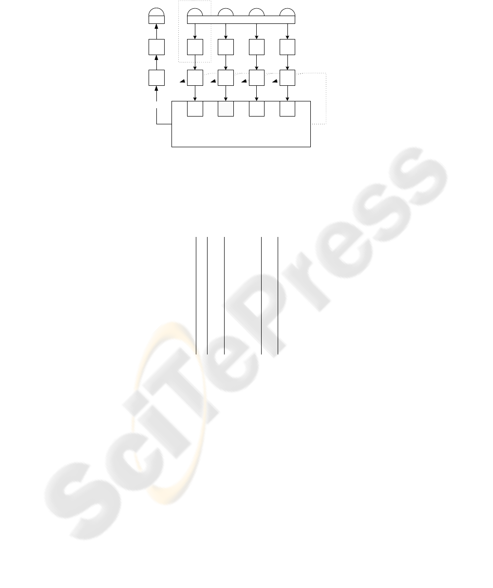
Sensor Board
TMS320F2812
US
0
US
1
US
2
US
3
Array
Amp.
&
BPF
Amp.
&
BPF
Amp.
&
BPF
Amp.
&
BPF
PGA
0
PGA
1
PGA
2
PGA
3
ADC
0
ADC
1
ADC
2
ADC
3
DAC
Amp.
UT
SPI
Fig.5. The goalkeper has an ultrasonic transmitter (UT) to send the broadcast signal and an
USS array with four receivers (USS
0
to USS
3
). The other robots have four pairs of transmit-
ters/receivers equally spaced around a circle.
Table 1. Anechoic chamber results: θ
r
- real angle, θ
m
- measured angle, ||θ
r
− θ
m
|| - absolute
error of the measured angle and σ
θ
m
- standard deviation for each angle.
θ
r
θ
m
||θ
r
− θ
m
|| σ
θ
m
-90° -83.63° 6.37° 1.90°
-80° -69.31° 10.69° 0.21°
-70° -68.55° 1.45° 0.37°
-60° -62.27° 2.27° 0.40°
-50° -36.11° 13.89° 0.22°
-40° -42.72° 2.72° 1.20°
-30° -34.95° 4.95° 0.14°
-20° -19.15° 0.85° 0.31°
-10° -8.73° 1.27° 0.24°
0° 0.36° 0.36° 0.24°
10° 9.53° 0.47° 0.50°
20° 24.54° 4.54° 0.43°
30° 43.11° 13.11° 0.88°
40° 39.45° 0.55° 0.23°
50° 42.59° 7.41° 0.18°
60° 47.49° 12.51° 0.79°
70° 69.31° 0.69° 0.21°
80° 70.66° 9.34° 0.37°
90° 83.86° 6.14° 2.32°
4 Experimental Results
Anechoic Chamber Tests. To gauge the localization system we tested it on two dif-
ferent situations, in an anechoic chamber and in a robot soccer field. In the anechoic
chamber we only tested the angle measurement in the -90° ≤ 0 ≤ 90° range using 10°
intervals with the transmitter at a distance of 7.5m. For each angle we took 5 measures.
The results of this test are shown in table 1.
In this experiment we observed that for angles between 30°and 60°the system was
very sensitive to small angle variations and that the received signal envelope was double
peaked due to multipath interference.
Robot Soccer Field Tests. We also performed localization tests in a robotics soccer
field. From this tests we got values for the absolute error position in a 1m grid for half

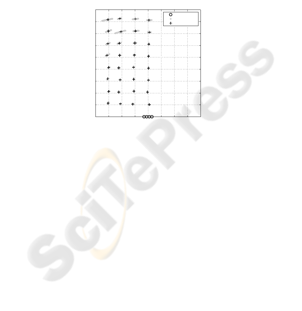
the field from 0 to -3m in the x coordinate and from 1 to 8m in the y coordinate. For each
position 50 measures were taken allowing the calculation of some statistical parameters
such as mean and the standard deviation of the measured distance and angle.
A X−Y plot with the test measurements and the estimated mean positions is shown
in figure 6.
−4 −3 −2 −1 0 1 2 3 4
0
1
2
3
4
5
6
7
8
9
X coordinate(m)
Y coordinate(m)
Sensor Array
Mesures
Mean
Fig.6. Position measures obtained in the soccer field with the USS array.
The error associated with the polar coordinates, distance and angle, of a position
test are presented in figures 7 a) and b). The distance has a maximum standard deviation
σ
d
m
= 1cm and the angle has a maximum standard deviation of σ
θ
m
= 1, 84°.
From the results shown in figure 6 it is observed that as the distance increases,
the variability of the measured position also increases. This can be explained by the
degradation of the signal to noise ratio of the received signals as the distance increases.
5 Conclusion
In this work we presented a complete system to localize soccer robots. An ultrasonic
sensor array combined with time data fusion, reduced the standard variance of the angle
measurements from 10° to 2°.
To improve the signal to noise ratio of the received signal (for large distances) the
system transmitted chirp pulses with a duration of 6.4ms. To be able to process the four
receiver channels simultaneously with a low cost DSP we implemented an efficient
baseband converter.

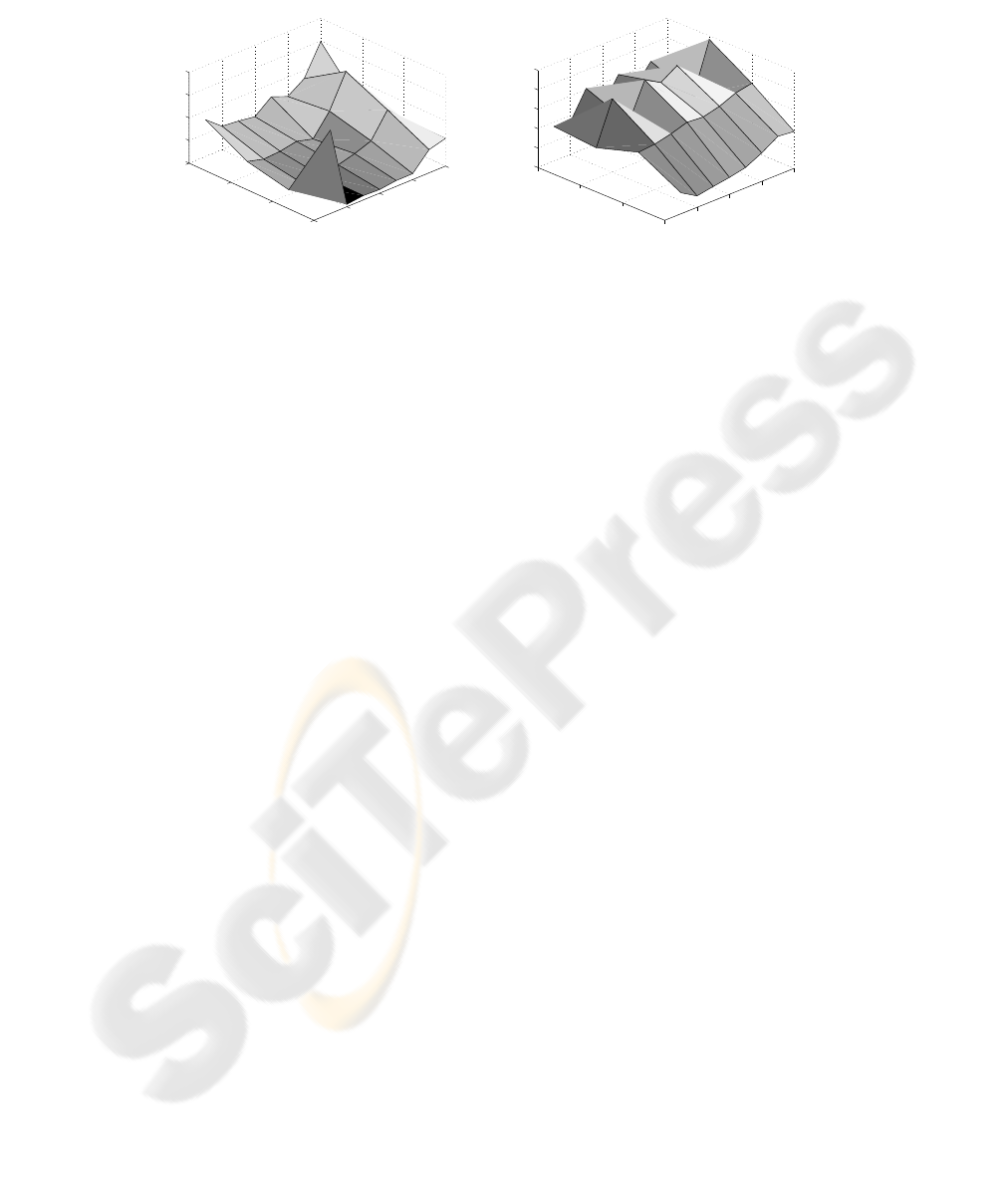
−3
−2
−1
0
0
2
4
6
8
0
0.5
1
1.5
2
Y coordinate (m)X coordinate (m)
σ
θ
m
(º)
(a) Angle
−3
−2
−1
00
2
4
6
8
0.05
0.1
0.15
0.2
0.25
0.3
Y coordinate (m)X coordinate (m)
||P
r
− P
m
|| (m)
(b) Position
Fig.7. Standard angle error and absolute position error.
References
1. Moravec, H.P., Elfes, A.: High resolution maps from wide angle sonar. In: Proceedings IEEE
International Conference on Robotics and Automation, Washington D. C., IEEE (1985) 116–
121
2. Elfes, A.: Sonar-based real world mapping and navigation. IEEE Transactions on Robotics
and Automation 4 (1987) 249–265
3. Sabatini, A.M., Spinielli, E.: Correlation techniques for digital time-of-flight measurement
by airborne ultrasonic rangefinders. In: Proceendings of the IROS’94, Munich, Germany
(1994)
4. Jrg, K.W., Berg, M.: Sophisticated mobile robot sonar sensing with pseudo-random codes.
Robotics and Autonomous Systems 25 (1998) 241–251
5. Vieira, J.M., Lopes, Srgio, I., Bastos, C.A.C., Fonseca, P.N.: Sistema de localizao utilizando
ultra-sons. In: Robtica 2006, Guimares, Portugal (2006)
6. Cook, C.E., Bernfeld, M.: Radar Signals - An Introduction to Theory and Application.
Artech House, Norwood (1993)
7. Sabatini, A.M., Rocchi, A.: Sampled baseband correlators for in-air ultrasonic rangefinders.
IEEE Transactions on Industrial Electronics 45 (1998) 341–350
8. Vaidyanathan, P.P.: Multirate Systems and Filter Banks. 1 edn. Signal Processing. Prentice-
Hall, New Jersey (1993)
9. Sayed, A.H., Tarighat, A., Khajehnouri, N.: Network-based wireless location. IEEE Signal
Processing Magazine 22 (2005) 24–40
10. Ko
ˇ
ci
ˇ
s, S., Figura, Z.: Ultrasonic Measurements and Technologies. Sensors Physics and
Technology. Chapman & Hall, London, UK (1996)