PC-SLIDING FOR VEHICLES PATH PLANNING

AND CONTROL

Design and Evaluation of Robustness to Parameters Change

and Measurement Uncertainty

Mariolino De Cecco, Enrico Bertolazzi, Giordano Miori, Roberto Oboe

Dep. Mech Struct Eng, University of Trento, Via Mesiano 77, Trento, Italy

Luca Baglivo

Dept. Mech. Eng., Universit of Padova, via Venezia 1, Padova, Italy

Keywords: Wheeled Mobile Robot, WMR, path generation, path control, nonholonomic, clothoid.

Abstract: A novel technique called PC-Sliding for path planning and control of non-holonomic vehicles is presented

and its performances analysed in terms of robustness. The path following is based upon a polynomial

curvature planning and a control strategy that replans iteratively to force the vehicle to correct for deviations

while sliding over the desired path. Advantages of the proposed method are its logical simplicity,

compatibility with respect to kinematics and partially to dynamics. Chained form transformations are not

involved. Resulting trajectories are convenient to manipulate and execute in vehicle controllers while

computed with a straightforward numerical procedure in real-time. The performances of the method that

embody a planner, a controller and a sensor fusion strategy is verified by Monte Carlo method to assess its

robustness to parameters changes and measurement uncertainties.

1 INTRODUCTION

Path generation and control is the problem of

determining a feasible set of commands that will

permit a vehicle to move from an initial state to a

final state following a desired geometrical figure in

space while correcting for deviations in real time.

While this problem can be solved for manipulators

by means of inverting nonlinear kinematics, the

common inverse problem for mobile robots is that of

inverting nonlinear differential equations.

A basic method is therefore to plan a geometric

path in the surface of motion, generally a 2D space,

and conceive a suitable control strategy to force the

vehicle to follow it. If the path is feasible its tracking

will be accurate, otherwise there will be non

negligible differences between the planned and the

executed path.

If one plan a continuous curvature path, than can

be sure of its compatibility with respect to

kinematics and partially to dynamics if the

maximum rate of curvature variation is taken into

consideration. This for a huge variety of vehicles. As

a matter of fact differential drive, car-like and all-

wheel steering vehicles have constraints in curvature

variation while moving.

Various methods have been employed to plan

smooth trajectories (Rodrigues 2003). Some of them

use splines (Labakhua 2006, Howard 2006, Solea

2006), other employ clothoids, generally in its linear

curvature representation, to concatenate straight line

segments with circumference arcs (Nagy 2000,

Labakhua 2006). To cope with more complex

representation of curvature, a method for trajectory

planning based upon parametric trajectory

representations have been developed (Kelly 2002).

The method employs a polynomial representation of

curvature. This is still a research field, obviously not

for the geometric representations in itself (Dubins

1957), for the definition of numerical algorithms and

control strategies efficiently employable in Real

Time and for the systematic investigation of their

robustness to parameters changes and measurement

uncertainties.

Starting from the method of Kelly, we optimised

the search strategy in order to extend the converging

De Cecco M., Bertolazzi E., Miori G., Oboe R. and Baglivo L. (2007).

PC-SLIDING FOR VEHICLES PATH PLANNING AND CONTROL - Design and Evaluation of Robustness to Parameters Change and Measurement

Uncertainty.

In Proceedings of the Fourth International Conference on Informatics in Control, Automation and Robotics, pages 11-18

DOI: 10.5220/0001634400110018

 SciTePress

solutions. We also added a control algorithm that is

perfectly integrated with the planning method.

The result is a Polynomial Curvature Sliding

control, PC-Sliding, a novel RT procedure for

planning and control that can be summarised as

follows. The steering commands are designed by

means of the polynomial curvature model applying a

two-point boundary value problem driven by the

differential posture (pose plus curvature). While

following the path the vehicle replans iteratively the

path with a repetition rate that must not necessarily

be deterministic. To the actual curvilinear coordinate

it is added a piece forward, than computed the

corresponding posture in the original planned path,

finally replanned the differential path steering the

vehicle from the actual posture to the one just

computed. The result is to force the vehicle to

correct for deviations while sliding over the desired

path. Those little pieces of correcting path have the

property of fast convergence, thanks also to an

optimised mathematical formulation, allowing a

Real Time implementation of the strategy.

Advantages of the proposed method are its

essentiality thanks to the use of the same strategy

both for planning and control. Controlling vehicles

in curvature assures compatibility with respect to

kinematics and partially to dynamics if the

maximum rate of curvature variation is taken into

consideration. The method doesn’t need chained

form transformations and therefore is suitable also

for systems that cannot be transformable like for

example non-zero hinged trailers vehicles (Lucibello

2001). Controls are searched over a set of admissible

trajectories resulting in corrections that are

compatible with kinematics and dynamics, thus

more robustness and accuracy in path following.

Resulting trajectories are convenient to manipulate

and execute in vehicle controllers and they can be

computed with a straightforward numerical

procedure in real-time. Disadvantages could be the

low degrees of freedom to plan obstacle-free path

(Baglivo 2005), but the method can readily be

integrated with Reactive Simulation methods (De

Cecco 2007), or the degree of the polynomial

representing curvature can be increased to cope

with those situations (Kelly 2002, Howard 2006).

Parametric trajectory representations limit

computation because they reduce the search space

for solutions but this at the cost of potentially

introducing suboptimality. The advantage is to

convert the optimal control formulation into an

equivalent nonlinear programming problem faster in

terms of computational load. Obviously the dynamic

model is not explicitly considered thus missing

effectiveness in terms of optimisation (Biral 2001).

By means of this iterative planning sliding

control strategy we obtain a time-varying control in

feedback which produces convergence to the desired

path, guaranteeing at the same time robustness. In

particular, small non-persistent perturbations are

rejected, while ultimate boundedness is achieved in

the presence of persistent perturbations.

Verification of stability convergence and

robustness can be achieved analytically or

statistically. The first way has the merit to synthesise

the results in a general and compact fashion. By

means of its analytic representation it is mostly easy

to isolate the influence parameters and quantify its

effect. The second way has the merit to cope easily

with complex models where interact different

effects. In the present paper we aim at verifying the

performances of the proposed method that embody a

planner, a controller and a sensor fusion strategy for

the vehicle pose estimation that takes into account

an iterative measurement system and an

environment referred one (De Cecco 2003, De

Cecco 2007). The fusion technique takes into

account also systematic effects. This last part

interacts with the control strategy injecting step

inputs of different entity at each fusion step. For the

above reasons we decided to take the second way of

verification employing a Monte Carlo method.

Generally research focuses on control or

measurement goal separately. Seldom the deep

interaction between them is taken into consideration.

In this work the whole system robustness is

investigated by simulation.

2 PATH PLANNING AND

CONTROL PROBLEMS

The main problem with Wheeled Mobile Robots

path planning and control tasks is well known and

it’s strictly related to the nonholonomic constraints

on velocity. These constraints limit possible

instantaneous movements of the robot and cause the

number of controlled states to be less than the

control inputs one. WMR state equations constitute

a non linear differential system that cannot be solved

in closed form in order to find the control inputs that

steer the robot from an initial to a goal posture

(position, heading and curvature). As a consequence

also the control task is non standard with respect to

the case of holonomic systems like the most part of

manipulators. A suitable control law for precise and

ICINCO 2007 - International Conference on Informatics in Control, Automation and Robotics

fast mobile robots path following should compute

feasible inputs that generate correcting paths

compliant with nonholonomic constraints.

2.1 Generalized Clothoids

Since the robot velocity vector (and therefore its

forward axis) has to be aligned with the path

tangent, it is natural and convenient to include the

curvature as a state while describing the robot state

equations. In fact the curvature is directly related to

the steering actuator input, therefore its continuity is

an important issue to prevent path following

deviations due to the planning phase.

A system state model that can be used for a car-

like or differential drive robot is:

() cos ()

() sin ()

() ()



ys s

sks

ks us

(1)

where the state vector (posture) consists of the

position coordinates x, y, heading

and curvature k.

Assuming, without losing generality, that k(s) is a

control input, the last equation in (1) can be omitted.

The derivatives are expressed with respect to the arc

length s rather than time, considering the robot

velocity as an independent input that doesn’t affect

the path geometry except for actuators dynamics

limitation.

Choosing for curvature a third order polynomial

in arc length allows to steer the robot from a given

starting to a final posture along a feasible smooth

path. In other words, the problem is that of

generating a continuous curvature path connecting

the two end-postures :

x( ) = [0 0 0 ]

x( ) [ ]=

fffff

s ,,,k

sx,y,δ ,k

(2)

The first constraint in equation (2) is anyway

general if the reference system is placed with its

origin at the initial position and oriented aligned

with the initial heading. In this way the first three

constraints are automatically satisfied and problem

is reduced to satisfy the remaining five constraints,

that is initial curvature and final posture.

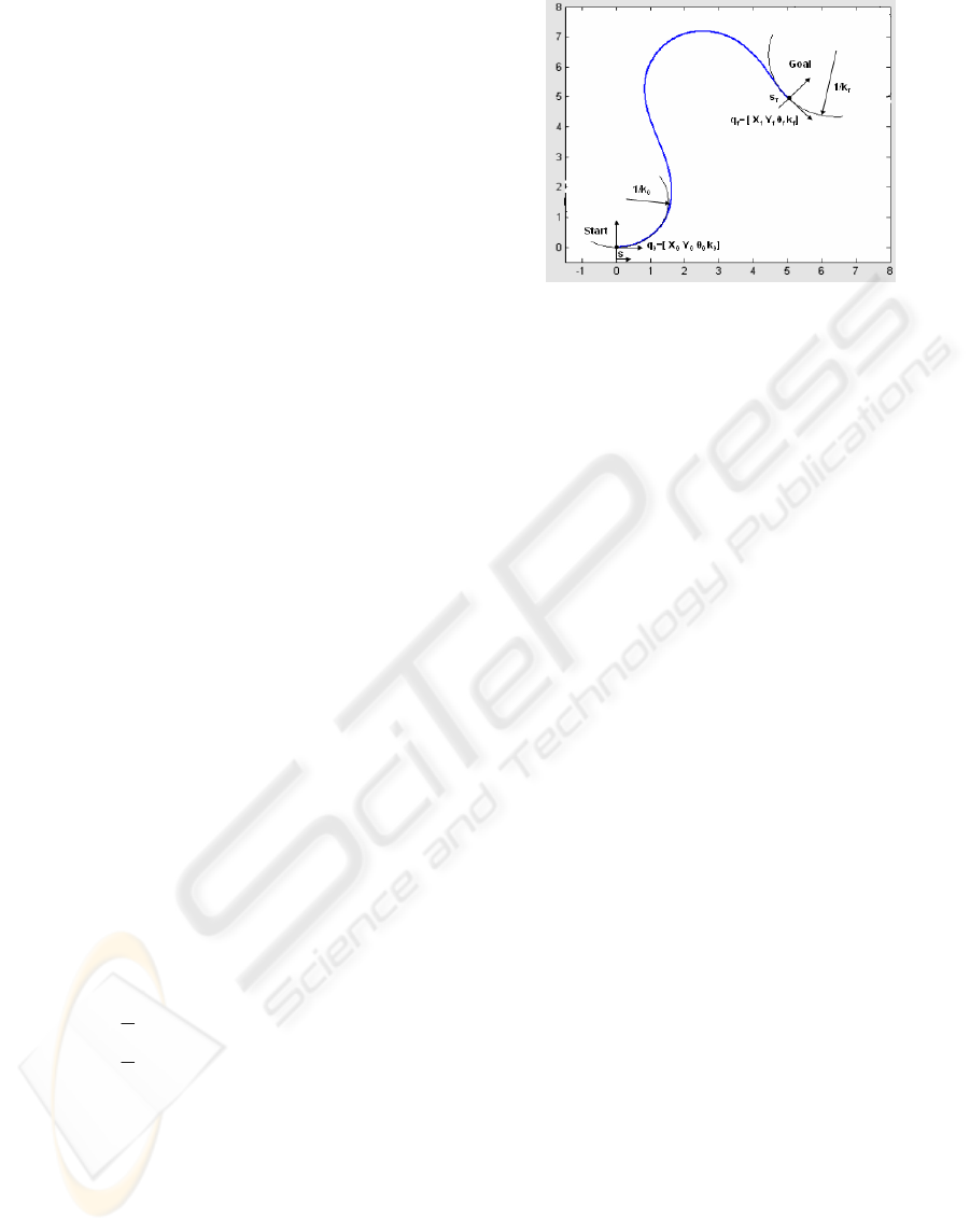
Figure 1: Continuous cubic curvature path planning. A

solution example.

The problem requires the solution of a nonlinear

differential equations system. In fact, while the

heading is obtained as a simple integration of the

curvature polynomial, the calculation of the

cartesian position [x, y] requires the numeric

integration of generalised Fresnel integrals. An

effort to solve the inverse two points boundary

problem (Figure 1) is worth thanks to the many

advantages that this formulation leads to. The aim is

to calculate five parameters, that in this case are the

four coefficients of the curvature polynomial, and

the total arc length s

. Once the calculation algorithm

has been designed and optimised, one could have, in

a few parameters, a representation of the planned

path that is nonholonomic compliant and can be

generated in real time. Examples can be an

autonomous path planning of a fork lift which have

to reach a detected pallet or to control a car in a fully

automated car parking. Besides, part of the solving

algorithm is exploited to generate the forward

integration of the curvature polynomial and the input

curvature can be applied to a large variety of WMR,

according to the kinematic model and dynamic

constraints, without changing the planning and

control algorithm.

3 THE PROPOSED METHOD

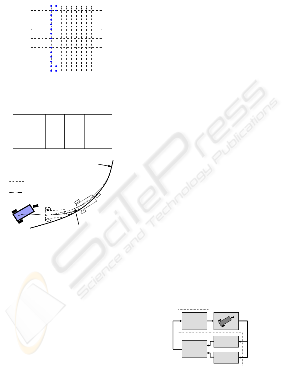
Starting from the method of (Kelly 2002), we

optimised the search strategy in order to extend the

converging solutions upon a large range of possible

final configurations (Figure 2).

The control algorithm we designed has revealed

to be efficient and very well integrated with the

planning method. It uses the same planning

algorithm to calculate feedback corrections,

asymptotically reducing servo errors to the reference

path.

PC-SLIDING FOR VEHICLES PATH PLANNING AND CONTROL - Design and Evaluation of Robustness to

Parameters Change and Measurement Uncertainty

-4 -3 -2 -1 0 1 2 3 4 5 6 7 8 9 10

-6

-4

-2

x[ m]

Y[ m]

Map of non converging solutions

Figure 2: Validation map of end postures without

convergence.

Table 1: Validation range.

Parameter Min Max Step

x 0 10 1 m

y -7 7 1 m

-π/2

π/2

0.1 rad

k -0.1 0.1 0.02 m

-1

path (k)

path (k+1)

path (k+2)

PC sliding

reference

path

k+1

k+2

path (k)

path (k+1)

path (k+2)

PC sliding

reference

path

k+1

k+2

Figure 3: Schematic representation of the control method.

At k·T

time-spaced instants a PC-sliding path is

computed to reach a sliding subtarget thus forcing the

robot to keep the desired planned PC path.

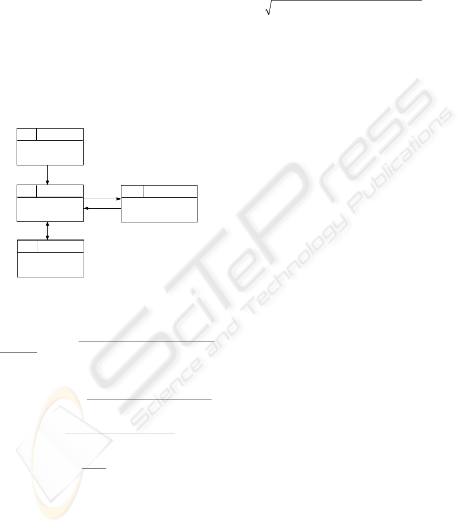
The whole algorithm can be summarized as

follows:

[Initialisation]

a) a reference PC path is planned, mapping the

arc length interval [0, s

] into the postures

[x(s), y(s),

(s), k(s)], that describe the robot

posture evolution from an initial posture

defined P

= [x

, y

, k

] to the final

desired posture P

= [x

, y

, k

] within

defined tolerances;

b) at initial condition the robot is placed in any

initial posture also different from P

;

c) if initial planning was successful (all

constraints satisfied), start moving at

constant velocity V.

[Loop at T

cycle time]

d) get actual position estimate and compute

the minimum distance position on the main

reference path and its corresponding arc

length s. Add to s an additional defined

length,

s, proportional to velocity.

If s +

s < s

= s +

s, otherwise s

= s

;

e) compute the correcting PC path by applying

point b) to plan a path between actual

posture and that mapped by s

on the

reference PC path [x(s

), y(s

( s

), k(s

)],

see Figure 3, path(k);

f) If s +

s > s

. Reduce velocity, set the

steering input according to the input

curvature k;

g) set the steering input according to the input

curvature k;

h) if final boundary condition is satisfied then

STOP;

i) GO TO point d)

4 IMPLEMENTATION

Real time feasibility was analyzed taking in mind

possible applications of industrial AGV transpallet.

The simulation tests, reported in §5.1, showed good

results in terms of fastness, low overall tracking

error and robustness. The RT implementation is at

the phase of Real Time cycle time verification and

architecture design.

4.1 Simulation

Simulations were carried out involving a three

wheeled robot (De Cecco 2003): 500 mm wheelbase

and a 50 mm front wheel radius. The path control

model incorporates the path planning and control.

The actuators dynamics is taken into account. A

model of a sensor fusion technique closes the loop

by feeding the current posture to the path controller

(see Figure 4). The sensor fusion algorithm

combines odometric and triangulating laser pose

estimates also taking into account systematic and

random effects (De Cecco 2007).

Odometric

Estimation

Sensor

Fusion

Laser

Estimation

Path

Control

Odometric

Estimation

Sensor

Fusion

Laser

Estimation

Path

Control

Figure 4: Logic scheme of the simulation model.

ICINCO 2007 - International Conference on Informatics in Control, Automation and Robotics

The simulated vehicle has two control inputs,

velocity and steering angle of the front wheel. The

actuators dynamics are simulated by means of first

order model with a time constant for the steering

mechanism of 0.1 s and that of the driving motor of

0.5 s. PC sliding method is updated with a refresh

cycle time T

of 0.015 seconds. A value of s

/20 for

Δs was used for driving velocity of 1.5 m/s.

4.2 RT Implementation

The PC-sliding algorithm was implemented on a

National Instruments 333 MHz PXI with embedded

real-time operating system (Pharlap).

Environment referred

me asu re men t

Tc=10

TAS K 1

[High Priority]

- POSE ESTIMATION

-Low level actuation

Tc=4

TAS K 3

[Critical Priority]

COM MUNICATION WITH

LASER

Tc=15

TASK 2

[Above Normal Priority]

PC-Sliding Path

Controller

Posture

Setpoint

Tc=50

TAS K 4

[Normal Priority]

COM MUNICATION WITH

CLIENT

User data

Figure 5: architecture for real time implementation.

The designed and preliminary verified software

architecture has four main tasks (see Figure 5):

• TASK 1 – Pose estimation & Low level

actuation: computes the best pose estimate starting

from odometers and laser data and computes the

reference commands to the drivers according to the

actual planned path.

• TASK 2 – PC-Sliding Path Controller

computes the corrective control action based upon

its current pose and the target one;

• TASK 3 – Communication with Laser

: acquires

the new pose measurement from laser when ready

and makes it available for task 1

• TASK 4 – Client

: communicates with a

reference station to manage the missions start-stop,

acquire and store data, etc.

The priority (static-priority) of the tasks was

assigned according to rate monotonic algorithm

which assign the priority of each task according to

its period, so that the shorter the period the higher

the priority.

Mean calculation times were measured for the

PC-sliding planning algorithm. After optimisation a

large number of paths were computed. The iteration

termination condition was triggered when a

weighted residual norm defined as:

22 22

()()( )()

xf yf f kf

rwx wy w wk

=Δ+Δ+Δ+Δ

(4)

is under a threshold of 0.001, and the weights are

computed in such a way that a fixed error upon final

or y

or k

, alone exceed the threshold. First

two weights in equation (4) were chosen equal to 1

-1

, last two weights were chosen to be equal to the

root square of ten. The computation time over all the

iterations showed in Figure 2 (only paths converging

under threshold) spanned from a minimum of

0.0003 to a maximum of 0.005 seconds. The

termination condition was thought to obtain a

feasible path for an industrial transpallet that has to

lift correctly a pallet.

5 VERIFICATION

In this work the whole system robustness is

investigated by simulation. We decided to evaluate

statistically rather than analytically the convergence

and the stability of the proposed method. The main

motivation is the aim to investigate not only the

influence of system delays and parameters bias on

the control, but also the interaction between a near-

reality measurement system used as the source of

feedback to the path controller. Monte Carlo

analysis is a powerful tool for this kind of tasks.

5.1 Simulation Results

Simulations were aimed at verifying control

robustness toward different aspects related to:

A. approximation of forward integration;

B. actuators delay and inaccuracy

C. non ideal initial conditions

D. control model parameters uncertainty

E. pose measurement noise

For all the tests the maximum following absolute

residual eps_path and final position residual eps_fin

were computed in meters.

A. The planned path is not an exact solution

because of generalized Fresnel integrals cannot be

solved in closed form and a reasonable computation

time is required for real time implementation.

Therefore a planning solution is accepted if the

termination condition is satisfied. First simulation

test was about verifying the vehicle model

implementation in ideal conditions, that is without

PC-SLIDING FOR VEHICLES PATH PLANNING AND CONTROL - Design and Evaluation of Robustness to

Parameters Change and Measurement Uncertainty

actuator dynamics, using nominal model parameters

and starting from ideal initial boundary conditions.

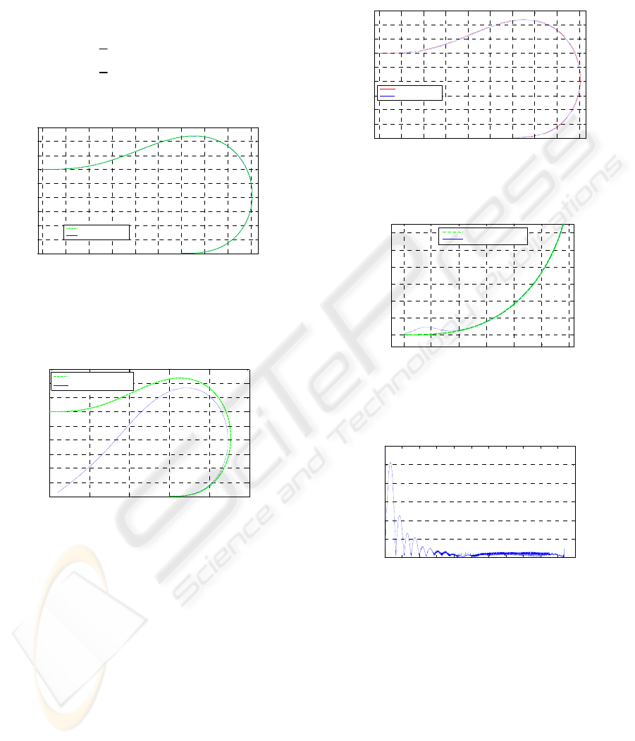
The path in Figure 6 has been chosen as the

representative path for the analysis. Boundary

conditions are:

x(0)=[0000]

x( ) [-6,3,π,0]=

,,,

(5)

-6 -5 -4 -3 -2 -1 0 1 2 3

0.5

1.5

2.5

3.5

4.5

Paths of Open Loop Simulation

x[m]

y[m]

Planned Path

Simulated True Path

Figure 6: open loop ideal path, only approximation affect

the following and final residual in this case.

eps_path= 0.007 m, eps_fin = 10

-4

m .

-6 -4 -2 0 2 4

0.5

1.5

2.5

3.5

4.5

Open Loop Path with Steering Bias and Dela

x[m]

y[m]

Planned Path

Simulated True Path

Figure 7: Open loop path with steering actuator biased and

delayed.

B. Without changing any condition with respect

to case A. except for the introduction of a dynamic

steering actuator model with a time constant of 0.1

seconds and a steering actuator bias of 1 degree the

resulting path is the one in Figure 7. To note that the

effect of the steering actuator is the most significant,

while the actuator delay effect is negligible. A proof

is that the simulated true path closes the bend more

than required.

Benefit of the proposed feedback controller can

be seen just making a comparison between the open

loop 1 degree steering angle biased case in Figure 7

and that in Figure 8 which is a result of close loop

applying in the case of 5 degree biased steering

actuation angle. The last could be considered a worst

case due to heavy mechanical skew or simply to bad

steering servo actuation. In this simulation the

residuals were eps_path = 0.026 m, eps_fin = 4·10

-4

-6 -5 -4 -3 -2 -1 0 1 2 3

0. 5

1. 5

2. 5

3. 5

4. 5

Closed loop with steering 5° bias and delay

x[ m]

y[m]

Planned Path

Simulated True Path

Figure 8: Close loop path with biased steering input angle

0 0.5 1 1.5 2 2.5 3

0.2

0.4

0.6

0.8

1.2

Initial Heading Error Simulation

x[ m]

y[m]

Planned Path

Simulated True Path

Figure 9: PC-sliding convergence to the reference path

starting from an initial heading of 15 degrees.

0 1 2 3 4 5 6 7 8 9 10 11

0. 02

0. 04

0. 06

0. 08

0. 1

0. 12

Time [s]

Foll owing Error [m]

Following Error VS Time

Figure 10: Residuals of the path following of the previous

figure.

C. Another significant simulation is the one

concerning with a non ideal initial condition: an

initial heading difference of 15 degree from the

aligned condition (Figure 9). In this case steering

delay is accounted too.

In Figure 10 it is showed that the following

absolute residual decreases asymptotically

remaining always bounded within reasonable values.

D. A set of simulations concerning the

robustness with respect to control parameters

uncertainties has been achieved. A Monte Carlo

approach was employed to analyse control

ICINCO 2007 - International Conference on Informatics in Control, Automation and Robotics

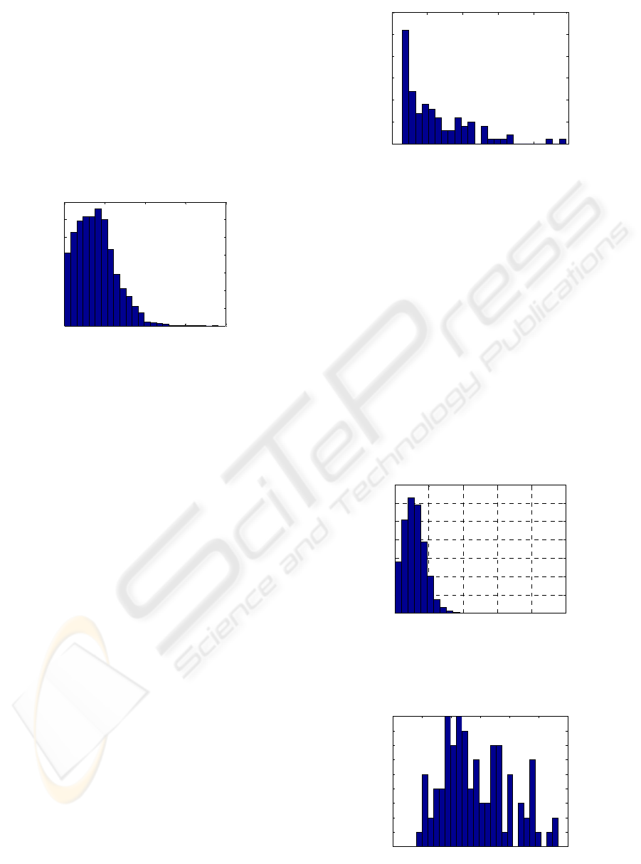
performances when an iterated randomized set of

control parameters is used to carry out a PC-sliding

path following task. More precisely, at each iteration

step the parameters b (wheelbase) and

(steering

angle for a theoretical straight path) are randomly

drawn from a normal unbiased distribution with

standard deviation σ

and σ

and then a complete

simulation, with same boundary constraints of the

previously presented cases, is done. Setting σ

0.002 m and σ

= 1 deg, the performance results are

those shown in Figure 11 and Figure 12.

0 0.005 0.01 0. 015 0.02

0.5

1.5

2.5

3.5

x 10

Error [m]

Occurency []

Path Following Residuals

Figure 11: Position residuals along each trial path

computed for each replan points at T

rate.

In this simulation the residuals were eps_path =

0.019 m, eps_fin = 10

-4

E. Last simulation tests are related to the

analysis of control robustness with respect to pose

measurement uncertainty. The first testing was made

by feeding simulated fused pose measurements to

the PC-sliding control algorithm. The measurement

simulation model involves a sensor fusion algorithm

that combines an odometric pose with a triangulating

laser estimate (see Figure 4). While the odometric

path estimate is smooth but affected by increasing

systematic errors with time, the laser sensor

furnishes unbiased but noisy pose measurements.

The sensor fusion algorithm compounds better

characteristic of the two measurement systems, but

the fused pose remains anyway affected by a certain

bias and by a certain noise. The parameters used for

the odometric model are the wheel radius R, the

wheelbase b and the steering angle offset α

. It was

set σ

= 0.002 m , σ

= 0.0005 m and σ

= 0.1 deg

for kinematic model parameters uncertainties. For

the laser pose measurement is reasonable to set the

standard deviation σ

= σ

0.015 m and that of

robot attitude as σ

= 0.002 rad. All the parameters

are ideal. Only the laser estimate is affected by noise

influencing the fused pose proportionally to

odometric uncertainty. Simulation residuals are

reported in Figure 13 and Figure 14. In this

simulation the residuals were eps_path = 0.024 m,

eps_fin = 0.013 m.

0 0.2 0.4 0.6 0.8 1

x 10

-4

Err or [ m]

Occurency []

End Point Residuals Histogram

Figure 12: End-point residuals, one for each trial path.

Finally we carried out a simulation set where all

the influencing factors were combined together. In

this case the odometric model was given random

parameters bias that were drawn randomly according

to those of the control model except for an

augmented steering actuation error, as such is

expected to be in reality. The parameters used by

odometric model were drawn from the same normal

distributions which were supposed to be in the

previous simulations set (σ

= 0.002 m , σ

= 0.0005

m and σ

= 0.1 deg) while the control model is

affected by the same wheelbase bias and by a 1

degree constant actuation error. In this simulation

the residuals were eps_path = 0.064 m, eps_fin =

0.028 m. In Figure 15 the worst case in term of

maximum following residual.

0 0.005 0. 01 0. 015 0. 02 0. 025

x 10

Error [m]

Occ urency []

Following Error

Figure 13: Position residuals along each path and for each

trial path in the case of measurement noise influence.

0 0.002 0.004 0. 006 0.008 0.01 0.012

Residuals [m]

Occurrency

End-Poi nt Residuals Histogram

Figure 14: End-point residuals, one for each trial path.

PC-SLIDING FOR VEHICLES PATH PLANNING AND CONTROL - Design and Evaluation of Robustness to

Parameters Change and Measurement Uncertainty

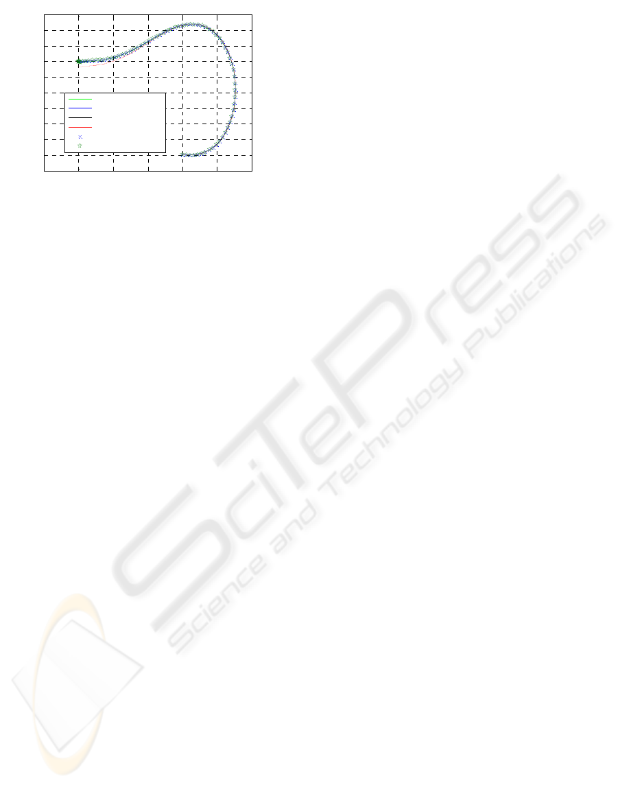
-8 -6 -4 -2 0 2 4

-0.5

0.5

1.5

2.5

3.5

4.5

Worst Case

x[ m]

y[m]

Planned Path

Simulated True Path

Fused Measure

Odometric Measure

Correct Measure

Laser Measure

Figure 15: Worst case in term of maximum following

residual in the combined influence factors simulations.

We would like to underline that in this

preliminary verification it was carried out a limited

number of iteration for the Monte Carlo analysis,

N = 100.

6 FUTURE WORK

Future work envisage an experimental verification

that will give an important verification of the

method effectiveness. Nevertheless simulation

results can be considered reliable from an in-

principle point of view (Baglivo 2005).

A second track of research foresee an increase of

the polynomial degree to achieve flexibility with

respect to obstacles constraints and minimum

curvature.

7 CONCLUSIONS

A novel technique for path planning and control of

non-holonomic vehicles is presented and its

performances verified. The performances of the

method that embody a planner, a controller and a

sensor fusion strategy was verified by Monte Carlo

simulation to assess its robustness to parameters

changes and measurement uncertainties.

The control algorithm showed high effectiveness

in path following also in presence of high

parameters deviations and measurement noise. The

overall performances are certainly compatible with

the operations of an autonomous transpallet for

industrial applications. Just to recall an example,

significant is the ability to compensate for a steering

error of 5° over a path of 180° attitude variation and

about 7 meters translation leading to a final

deviation of only 0.5 mm in simulation.

REFERENCES

Baglivo L., De Cecco M., Angrilli F., Tecchio F., Pivato

A., 2005 An integrated hardware/software platform

for both Simulation and Real-Time Autonomus Guided

Vehicles Navigation, ESM, Riga, Latvia, June 1st -

4th.

Biral F., Da Lio M., 2001 Modelling drivers with the

Optimal Manoeuvre method, ATA Congress, firenze

2001, 01A1029, 23-25 May.

De Cecco M., Baglivo L., Angrilli F., 2007 Real-Time

Uncertainty Estimation of Autonomous Guided

Vehicles Trajectory taking into account Correlated

and Uncorrelated Effects, IEEE Transactions on

Instrumentation and Measurement.

De Cecco M., Marcuzzi E., Baglivo L., Zaccariotto M.,

2007 Reactive Simulation for Real-Time Obstacle

Avoidance, Informatics in Control Automation and

Robotics III, Springer.

De Cecco M., 2003 Sensor fusion of inertial-odometric

navigation as a function of the actual manoeuvres of

autonomous guided vehicles, Measurement Science

and Technology, vol. 14, pp 643-653.

Dubins L. E., 1957 On Curves of Minimal Length with a

Constraint on Average Curvature and with Prescribed

Initial and Terminal Positions and Tangents,

American Journal of Mathematics, 79:497- 516.

Howard T., Kelly A., 2006 Continuous Control Primitive

Trajectory Generation and Optimal Motion Splines for

All-Wheel Steering Mobile Robots, IROS.

Kelly A., Nagy B., 2002. Reactive Nonholonomic

Trajectory Generation via Parametric Optimal

Control, International Journal of Robotics Research.

Labakhua L., Nunes U., Rodrigues R., Leite F. 2006.

Smooth Trajectory planning for fully automated

passengers vehicles, Third International Conference

on Informatics in Control, Automation and Robotics,

ICINCO.

Leao D., Pereira T., Lima P., Custodio L. 2002 Trajectory

planning using continuous curvature paths, DETUA

Journal, vol 3, n° 6.

Lucibello P., Oriolo G., 2001. Robust stabilization via

iterative state steering with an application to chained-

form systems, Automatica vol. 37, pp 71-79.

Nagy, M. and T. Vendel , 2000. Generating curves and

swept surfaces by blended circles. Computer Aided

Geometric Design, Vol. 17, 197-206.

Solea, R., Nunes U., 2006. Trajectory planning with

embedded velocity planner for fully-automated

passenger vehicles. IEEE 9th Intelligent

Transportation Systems Conference. Toronto, Canada.

Rodrigues, R., F. Leite, and S. Rosa, 2003. On the

generation of a trigonometric interpolating curve in

ℜ

, 11th Int. Conference on Advanced Robotics,

Coimbra, Portugal.

ICINCO 2007 - International Conference on Informatics in Control, Automation and Robotics