
Cooperative Collision Avoidance between Multiple
Robots based on Bernstein-B
´
ezier Curves
Igor
ˇ
Skrjanc and Gregor Klan
ˇ
car
Faculty of Electrical Engineering, University of Ljubljana
Tr
ˇ
za
ˇ
ska 25, SI-1000 Ljubljana, Slovenia
Abstract. In this paper a new cooperative collision-avoidance method for mul-
tiple nonholonomic robots based on Bernstein- B
´
ezier curves is presented. The
reference path of each robot from the start pose to the goal pose, is obtained
by minimizing the penalty function, which takes into account the sum of all the
paths subjected to the distances between the robots, which should be bigger than
the minimal distance defined as the safety distance. When the reference paths
are defined the model predictive trajectory tracking is used to define the control.
A prediction model derived from linearized tracking-error dynamics is used to
predict future system behavior. A control law is derived from a quadratic cost
function consisting of the system tracking error and the control effort. The results
of the simulation and some future work ideas are discussed.
1 Introduction
Collision avoidance is one of the main issues in applications for a wide variety of tasks
in industry, human-supported activities, and elsewhere. Often, the required tasks cannot
be carried out by a single robot, and in such a case multiple robots are used coop-
eratively. The use of multiple robots may lead to a collision if they are not properly
navigated. Collision-avoidance techniques tend to be based on speed adaptation, route
deviation by one vehicle only, route deviation by both vehicles, or a combined speed
and route adjustment. When searching for the best solution that will prevent a collision
many different criteria are considered: time delay, total travel time, planned arrival time,
etc. Our optimality criterion will be the minimal travel time, which directly implies a
minimal total length of the robot paths, subject to a minimal safety distance between all
the robots.
In the literature many different techniques for collision avoidance have been pro-
posed. The first approaches proposed avoidance, when a collision between robots is
predicted, by stopping the robots for a fixed period or by changing their directions.
The combination of these techniques is proposed in [1]. The behavior-based motion
planning of multiple mobile robots in a narrow passage is presented in [2]. Intelligent
learning techniques were incorporated into neural and fuzzy control for mobile-robot
navigation to avoid a collision as proposed in [3].
In our paper the control of multiple mobile robots to avoid collisions in a two-
dimensional free-space environment is separated into the path planning for each indi-
vidual robot to reach its goal pose as fast as possible. The second part of the task is to
design the control that will ensure the perfect trajectory tracking of the mobile robots.
ˇ
Skrjanc I. and Klan
ˇ
car G. (2007).
Cooperative Collision Avoidance between Multiple Robots based on Bernstein-B
´
ezier Curves.
In Proceedings of the 3rd International Workshop on Multi-Agent Robotic Systems, pages 34-43
Copyright
c
SciTePress

Several controllers were proposed for mobile robots with nonholonomic constraints.
An extensive review of nonholonomic control problems can be found in [4]. In trajectory-
tracking control a reference trajectory is usually obtained by using a reference robot;
therefore, all kinematics constraints are implicitly considered by a reference trajectory.
From the reference trajectory a feed-forward system of inputs combined with a feed-
back control law are mostly used [5]. Lyapunov stable time-varying state-tracking con-
trol laws were pioneered by [9]. The stabilization to the reference trajectory requires
a nonzero motion condition. Many variations and improvements to this state-tracking
controller followed in subsequent research [10]. A tracking controller obtained with
input-output linearization is used in [5], a saturation feedback controller is proposed in
[11] and a dynamic feedback linearization technique is used in [6].
The paper is organized as follows. In Section 2 the problem is stated. The concept
of path planning is shown in Section 3. The idea of optimal collision avoidance for
multiple mobile robots based on B
´
ezier curves is discussed in Section 4. The trajectory-
tracking controller design where the control strategy consists of feed-forward and feed-
back actions is introduced in Section 5. In Section 5.1 the proposed model predictive
controller is derived. The simulation results of the obtained collision-avoidance control
are presented in Section 6 and the conclusion is given in Section 7.
2 Statement of the Problem
The collision-avoidance control problem of multiple nonholonomic mobile robots is
proposed in a two-dimensional free-space environment. The simulations are performed
for a small two-wheel differentially driven mobile robot of dimension 7.5 × 7.5 × 7.5
cm. The architecture of our robots has a nonintegrable constraint in the form ˙x sin θ −
˙y cos θ = 0 resulting from the assumption that the robot cannot slip in a lateral direction
where q(t) = [x(t) y(t) θ(t)]
T
are the generalized coordinates The kinematics model
of the mobile robot is
˙q (t) =
cos θ(t) 0
sin θ(t) 0
0 1
v(t)
ω(t)
(1)
where v(t) and ω(t) are the tangential and angular velocities of the platform. During
low-level control the robot’s velocities and accelerations are bounded within the maxi-
mal allowed velocities and accelerations, which prevents the robot from slipping.
The danger of a collision between multiple robots is avoided by determining the
strategy of the robots’ navigation, where we define the reference path to fulfil certain
criteria. The reference path of each robot from the start pose to the goal pose is obtained
by minimizing the penalty function, which takes into account the sum of all the paths
subjected to the distances between the robots, which should be larger than the defined
safety distance. When the reference paths are defined the model predictive trajectory
tracking is used to define the control.

3 Path Planning based on Bernstein-B
´
ezier Curves
Given a set of control points P
0
, P
1
, . . . , P
b
, the corresponding Bernstein-B
´
ezier curve
(or B
´
ezier curve) is given by
r(λ) =
b
X
i=0
B
i,b
(λ)p
i
where B
i,b
(λ) is a Bernstein polynomial, λ is a normalized time variable (λ = t/T
max
,
0 ≤ λ ≤ 1) and p
i
, 0 = 1, . . . , b stands for the local vectors of the control point P
i
(p
i
= P
i
x
e
x
+ P
i
y
e
y
, where P
i
=
P
i
x
, P
i
y
is the control point with coordinates P
i
x
and P
i
y
, and e
x
and e
y
are the corresponding base unity vectors). The Bernstein-B
´
ezier
polynomials, which are the base functions in the B
´
ezier-curve expansion, are given as
follows:
B
i,b
(λ) =
b
i
λ
i
(1 − λ)
b−i
, i = 0, 1, . . . , b
which have the following properties: 0 ≤ B
i,b
(λ) ≤ 1, 0 ≤ (λ) ≤ 1 and
P
b
i=0
B
i,b
=
1.
The B
´
ezier curve always passes through the first and last control point and lies
within the convex hull of the control points. The curve is tangent to the vector of the
difference p
1
− p
0
at the start point and to the vector of the difference p
b
− p
b−1
at the
goal point. A desirable property of these curves is that the curve can be translated and
rotated by performing these operations on the control points. The undesirable properties
of B
´
ezier curves are their numerical instability for large numbers of control points, and
the fact that moving a single control point changes the global shape of the curve. The
former is sometimes avoided by smoothly patching together low-order B
´
ezier curves.
The properties of B
´
ezier curves are used in path planning for nonholonomic mobile
robots. In particular, the fact of the tangentiality at the start and at the goal points and
the fact that moving a single control point changes the global shape of the curve. Let us
assume the starting pose of the mobile robot is defined in the generalized coordinates
as q
s
= [x
s
, y
s
, θ
s
]
T
and the goal pose is defined as q
g
= [x
g
, y
g
, θ
g
]
T
, which means
that the robot starts in position P
s
(x
s
, y
s
) with orientation θ
s
and has a goal defined
with position P
g
(x
g
, y
g
) with orientation θ
g
. The property of tangentiality requires the
definition of the neighboring points P
1
(x
1
, y
1
) and P
2
(x
2
, y
2
), which become
P
1
(x
s
+ d cos θ
s
, y
s
+ d sin θ
s
), P
2
(x
g
+ d cos (θ
g
+ π), y
g
+ d sin (θ
g
+ π)) (2)
where d stands for the distance between P
s
and P
1
and between P
g
and P
2
. The distance
d is usually defined relatively to the distance between the start and the goal point D
(D =| p
g
− p
s
|) defined as d = γD, 0 < γ < 0.5. These four control points P
s
,
P
1
, P
2
and P
g
uniformly define the third order B
´
ezier curve. The need for flexibility
of the global shape and the fact that moving a single control point changes the global
shape of the curve imply the introduction of another point, which will be denoted as
P
o
(x
o
, y
o
). By changing the position of point P
o
the global shape of the curve changes.
This means that having in mind the flexibility of the global shape of the curve and the
start and the goal pose of the mobile robot, the path can be planned by four fixed points
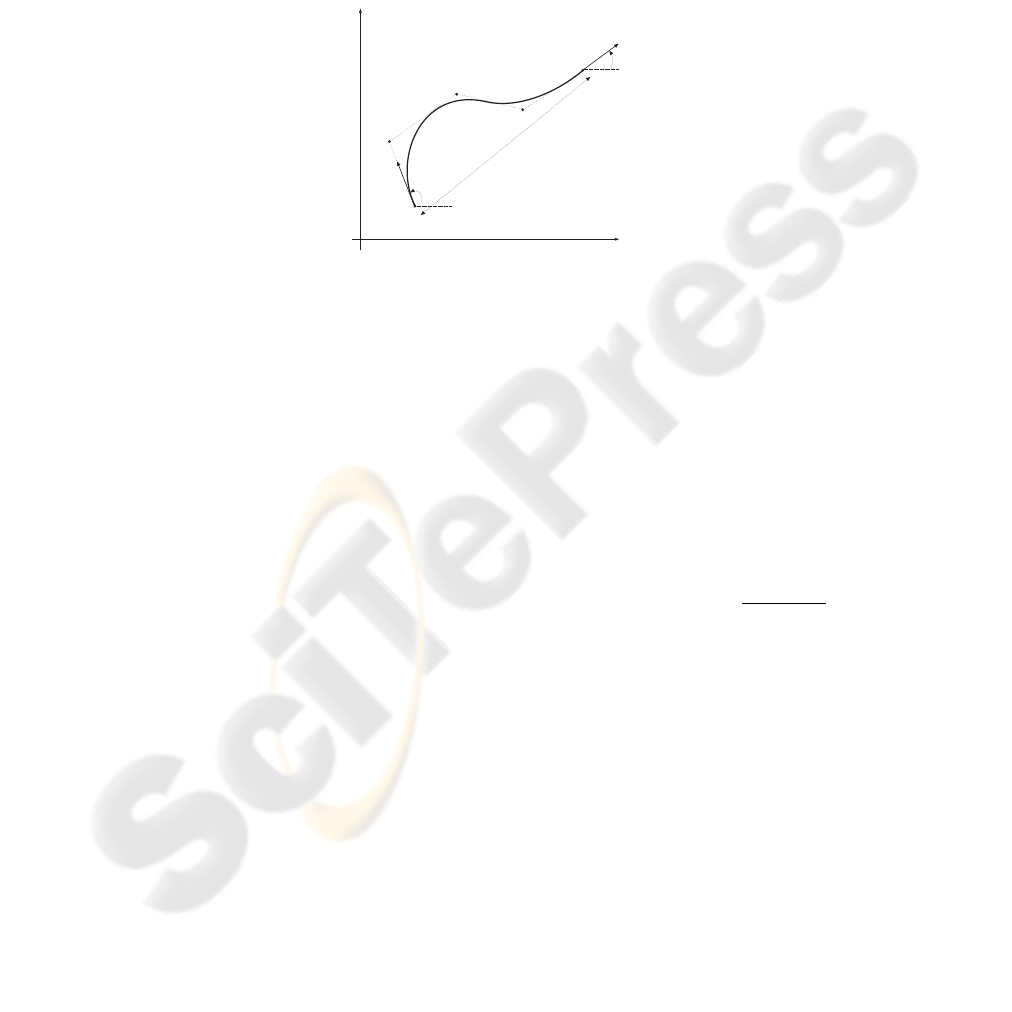
and one variable point. The B
´
ezier curve is now defined as a sequence of points P
s
, P
1
,
P
o
, P
2
and P
g
in Fig 1. This means that we are dealing with Bernstein polynomials of
the fourth order (B
i,b
, i = 0, . . . , b, b = 4). The curve is defined as follows:
r(λ) = B
0,4
p
s
+ B
1,4
p
1
+ B
2,4
p
o
+ B
3,4
p
2
+ B
4,4
p
g
(3)
y
x
P xy
1 1 1
( , )
P x y
s s s
( , )
P xy
o o o
( , )
P xy
2 2 2
( , )
P xy
g g g
( , )
q
g
q
s
D
Fig.1. The B
´
ezier curve.
4 Optimal Collision Avoidance based on Bernstein-B
´
ezier Curves
In this subsection a detailed presentation of cooperative multiple robots collision avoid-
ance based on B
´
ezier curves will be given. Let as assume the number of robots equals
n. The i-th robot is denoted as R
i
and has the start position defined as P
si
(x
si
, y
si
)
and the goal position defined as P
g i
(x
g i
, y
g i
). The reference path of i-th robot will be
denoted with the B
´
ezier curve r
i
(λ) = [x
i
(λ), y
i
(λ)]
T
. By choosing maximal time of
the experiment T
max
(t = T
max
λ, 0 ≤ λ ≤ 1) the robots tangential velocity profiles
are determined. T
max
is determined by the fastest robot R
i
as T
max
=
max
i
(v
i
(λ))
v
max
,
i = 1, . . . , n, 0 ≤ λ ≤ 1, where v
max
is maximal allowed tangential robot velocity.
Maximal time T
max
is then common to all robots R
i
. In Fig. 2 a collision avoidance for
n = 2 is presented for reasons of simplicity.
The safety margin to avoid a collision between two robots is, in this case, defined
as the minimal necessary distance between these two robots. The distance between the
robot R
i
and R
j
is r
ij
(λ) =| r
i
(λ) − r
j
(λ) |, i = 1, . . . , n, j = 1, . . . , n, i 6= j.
Defining the minimal necessary safety distance as d
s
, the following condition for
collision avoidance is obtained r
ij
≥ d
s
, 0 ≤ λ ≤ 1, i, j. Fulfilling this criteria means
that the robots will never meet in the same region defined by a circle with radius d
s
,
which is called a non-overlapping criterion. At the same time we would like to minimize
the length of the path for each robot, which is defined as s
i
. The length s
i
(λ) is defined
as s
i
(λ) =
R
λ
0
v
i
(λ)dλ, where v
i
(λ) stands for the tangential velocity in the normalized
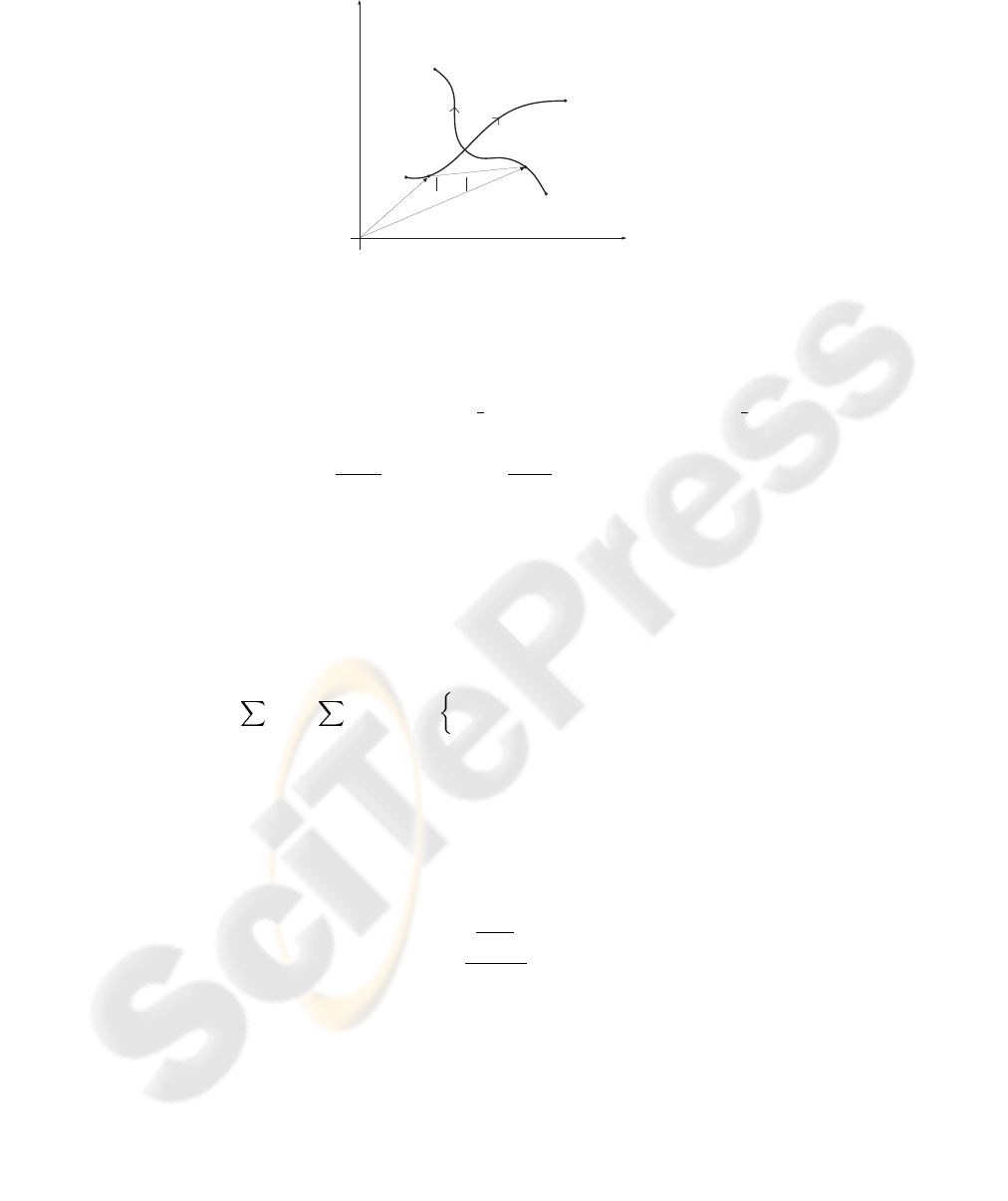
y
x
P xy
g g g1 1 1
( , )
P x y
s s s1 1 1
( , )
P x y
s s s2 2 2
( , )
P xy
g g g2 2 2
( , )
1
( )lr
2
( )lr
1 2
-r r
Fig.2. Collision avoidance based on Bernstein-B
´
ezier.
variable λ and the length of the path of the robot R
i
from the start control point to the
goal point is now calculated as:
v
i
(λ) =|
˙
r(λ) |=
˙x
2
i
(λ) + ˙y
2
i
(λ)
1
2
, s
i
=
Z
1
0
( ˙x
2
i
(λ)) + ˙y
2
i
(λ))
1
2
dλ
where ˙x
i
(λ) stands for
dx
i
(λ)
dλ
and ˙y
i
(λ) for
dy
i
(λ)
dλ
. Assuming that the start and goal
control points are known, the global shape and length of each path can be optimized by
changing the flexible control point P
oi
. The collision-avoidance problem is now defined
as an optimization problem as follows:
minimize
n
X
i=1
s
i
subject to d
s
− r
ij
(λ) ≤ 0, ∀i, j, i 6= j, 0 ≤ λ ≤ 1 (4)
The minimization problem is called an inequality optimization problem and can be
introduced as the minimization of the following penalty function
F (P
o
) =
i
s
i
+ c
ij
Γ
ij
, Γ
ij
=
1, min r
ij
(λ) < d
s
0, min r
ij
(λ) > d
s
, i, j, i 6= j, 0 ≤ λ ≤ 1 (5)
where c stands for a large scalar to penalize the unfulfillment of constraints. The
solution of the minimization problem min
P
o
F is a set of n control points P
o
=
{P
o1
, . . . , P
on
}. Each optimal control point P
oi
, i = 1, . . . , n uniformly defines one
optimal path, which ensures collision avoidance in the sense of a safety distance and
will be used as a reference trajectory of the ith robot and will be denoted as r
ri
(λ).
To define the feasible reference path that will be collision safe, the real time should
be introduced. In the real system the tangential and the angular velocities are limited to
(v
max
, ω
max
). Using the relation v(t) =
v(λ)
T
max
the maximal time T
max
can be defined
to fulfil the velocity limitation (T
max
≥
max v(λ)
v
max
).
5 Path Tracking
The previously obtained optimal collision-avoidance path for the ith robot is defined as
r
ri
(t) = [x
ri
(t), y
ri
(t)]
T
, i = 1, . . . , n. In this section the development of a predictive

path-tracking controller will be presented. The path-tracking control is realized as a sum
of the feed-forward and feed-back controls. The feed-forward control for the ith robot
is calculated from a feasible reference path r
ri
(t) = [x
ri
(t), y
ri
(t)]
T
, which enables us
to reach a desired pose. The feed-forward control inputs v
ri
(t) and ω
ri
(t) are derived
using a kinematic model (1). The tangential velocity v
ri
(t) and the tangent angle of
each point on the path are calculated as follows
v
ri
(t) =
˙x
2
ri
(t) + ˙y
2
ri
(t)
1
2
, ω
ri
(t) =
˙x
ri
(t)¨y
ri
(t) − ˙y
ri
(t)¨x
ri
(t)
˙x
2
ri
(t) + ˙y
2
ri
(t)
= v
ri
(t)κ(t)
(6)
where κ(t) is the path curvature. The necessary condition in the path-design procedure
is a twice-differentiable path and a nonzero tangential velocity v
ri
(t) 6=0.
If for some time t the tangential velocity is v
ri
(t)=0, the robot rotates at a fixed
point with the angular velocity ω
ri
(t) calculated from an explicitly given θ
ri
(t).
The feedback control law is derived from a linear time-varying system obtained by
an approximate linearization around the trajectory. The obtained linearization is shown
to be controllable as long as the trajectory does not come to a stop, which implies that
the system can be asymptotically stabilized by smooth time-varying linear or nonlinear
feedback. The tracking error e(t) = [e
1
(t) e
2
(t) e
3
(t)]
T
of a mobile robot expressed in
the frame of the real robot reads
e =
cos θ sin θ 0
− sin θ cos θ 0
0 0 1
(q
ri
− q) . (7)
Considering the robot kinematics (1) and derivating relations (7) the following kine-
matics model is obtained
˙
e =
cos e
3
0
sin e
3
0
0 1
v
ri
ω
ri
+
−1 e
2
0 −e
1
0 −1
u (8)
where u = [v ω]
T
is the velocity input vector and v
ri
and ω
ri
are already defined in (6).
The robot input vector u is further defined as the sum of the feed-forward and feedback
control actions (u = u
F
+ u
B
) where the feed-forward input vector, u
F
, is obtained
by a nonlinear transformation of the reference inputs u
F
= [v
ri
cos e
3
ω
ri
]
T
and the
feedback input vector, is u
B
= [u
B
1
u
B
2
]
T
, which is the output of the controller defined
in section 5.1.
Using the relation u = u
F
+ u
B
, rewriting (8) and furthermore, by linearizing the
error dynamics around the reference trajectory (e
1
= e
2
= e
3
= 0, u
B
1
= u
B
2
= 0)
the following linear model is obtained
˙
e =
0 ω
ri
0
−ω
ri
0 v
ri
0 0 0
e +
−1 0
0 0
0 −1
u
B
(9)
which in the state-space form is
˙
e = A
c
e + B
c
u
B
. According to Brockett’s condition
[12] a smooth stabilization of the system (1) or its linearization is only possible with
time-varying feedback. In the following the obtained linear model is used in the derived
predictive control law.

5.1 Model Predictive Control based on a Robot Tracking-error Model
To design the controller for trajectory tracking the system (9) will be written in discrete-
time form as
e(k + 1) = Ae(k) + Bu
B
(k)
where A ∈ R
n
× R
n
, n is the number of state variables and B ∈ R
n
× R
m
, m is the
number of input variables. The discrete matrix A and B can obtained as follows:A =
I + A
c
T
s
, B = B
c
T
s
which is a good approximation during a short sampling time
T
s
.
The idea of the moving-horizon control concept is to find the control-variable values
that minimize the receding-horizon quadratic cost function (in a certain interval denoted
with h) based on the predicted robot-following error:
J(u
B
, k) =
h
X
i=1
ǫ
T
(k, i)Qǫ(k, i) + u
T
B
(k, i)Ru
B
(k, i) (10)
where ǫ(k, i) = e
ri
(k + i) − e(k + i|k) and e
ri
(k + i) and e(k + i|k) stands for the
reference robot following-trajectory and the robot-following error, respectively, and Q
and R stand for the weighting matrices where Q ∈ R
n
× R
n
and R ∈ R
m
× R
m
, with
Q ≥ 0 and R ≥ 0.
Output prediction in the discrete-time framework In the moving time frame the
model output prediction at the time instant h can be written as:
e(k + h|k) = Π
h−1
j=1
A(k + j|k)e(k) +
P
h
i=1
Π
h−1
j=i
A(k + j|k)
B(k + i − 1|k)·
·u
B
(k + i − 1) + +B(k + h − 1|k)u
B
(k + h − 1) .
(11)
Defining the robot-tracking prediction-error vector
E
∗
(k) =
e(k + 1|k)
T
e(k + 2|k)
T
. . . e(k + h|k)
T
T
where E
∗
∈ R
n·h
for the whole interval of observation (h) and the control vector
U
B
(k) =
u
T
B
(k) u
T
B
(k + 1) . . . u
T
B
(k + h − 1)
T
and
Λ
Λ
Λ(k, i) = Π
h−1
j=i
A(k + j|k)
the robot-tracking prediction-error vector is written in the form
E
∗
(k) = F(k)e(k) + G(k)U
B
(k) (12)
where
F(k) = [A(k|k) A(k + 1|k)A(k|k) . . . Λ
Λ
Λ(k, 0)]
T
, (13)
and G(k) = [g
ij
] , i = 1, ..., n, j = 1, ..., b, b = max(h, n), g
11
= B(k |k),g
21
=
A(k+1|k)B(k|k), g
22
= B(k+1|k), g
n1
= Λ
Λ
Λ(k, 1)B(k|k), g
n2
= Λ
Λ
Λ(k, 2)B(k+1|k),
g
nh
= B(k + h − 1|k). and F(k) ∈ R
n·h
× R
n
, G(k) ∈ R
n·h
× R
m·h
.

The objective of the control law is to drive the predicted robot trajectory as close
as possible to the future reference trajectory, i.e., to track the reference trajectory. This
implies that the future reference signal needs to be known. Let us define the reference
error-tracking trajectory in state-space as e
ri
(k + i) = A
i
ri
e(k). for i = 1, . . . , h. This
means that the future control error should decrease according to dynamics defined with
the reference model matrix A
ri
. Defining the robot reference-tracking error vector
E
∗
ri
(k) =
e
ri
(k + 1)
T
e
ri
(k + 2)
T
. . . e
ri
(k + h)
T
T
, E
∗
ri
∈ R
n·h
for the whole interval of observation (h) the following is obtained
E
∗
ri
(k) = F
ri
e(k), F
ri
=
A
ri
A
2
ri
. . . A
h
ri
T
, F
ri
∈ R
n·h
× R
n
. (14)
Control law The idea of MPC is to minimize the difference between the predicted
robot-trajectory error and the reference robot-trajectory error in a certain predicted in-
terval.
The cost function is, according to the above notation, now written as
J(U
B
) = (E
∗
ri
− E
∗
)
T
Q (E
∗
ri
− E
∗
) + U
T
B
RU
B
. (15)
The control law is obtained by the minimization (
∂J
∂U
B
= 0) of the cost function and
becomes
U
B
(k) =
G
T
QG + R
−1
G
T
Q (F
ri
− F) e(k) (16)
where
Q = diag(Q) and R = diag(R). This means that Q ∈ R
n·h
× R
n·h
and
R ∈ R
m·h
× R
m·h
.
Let us define the first m rows of the matrix
G
T
QG + R
−1
G
T
Q (F
ri
− F) ∈
R
m·h
× R
n
as K
mpc
. Now the feedback control law of the model predictive control is
given by
u
B
(k) = K
mpc
· e(k), K
mpc
∈ R
m
× R
n
(17)
6 Simulation Results
In this section the simulation results of the optimal cooperative collision avoidance
between three mobile robots are shown. The study was made to elaborate the possible
use in the case of a real mobile-robot platform. In the real platform we are faced with
the limitation of control velocities and accelerations. The maximal allowed tangential
velocity and angular velocity were v
max
= 0.5 m/s and ω
max
= 13 rad/s, while the
maximal allowed tangential wheel acceleration is a
max
= 3m/s
2
. Because of relatively
hight maximal angular velocity and tangential wheel acceleration only the tangential
velocity was taken into account to define the maximal time between the start position
of the robots and the goal position, which is defined as T
max
≥
max v(λ)
v
max
=
2.1m
0.5ms
−1
=
4.02s where the maximal normalized tangential velocity max
i
v
i
(λ) = 2.1m is defined
from Fig. 3. The starting pose of the first mobile robot R
1
in generalized coordinates is
defined as q
s1
=
0, 1,
π
2
T
and the goal pose as q
g 1
=
1, 0, −
π
4
T
. The second robot
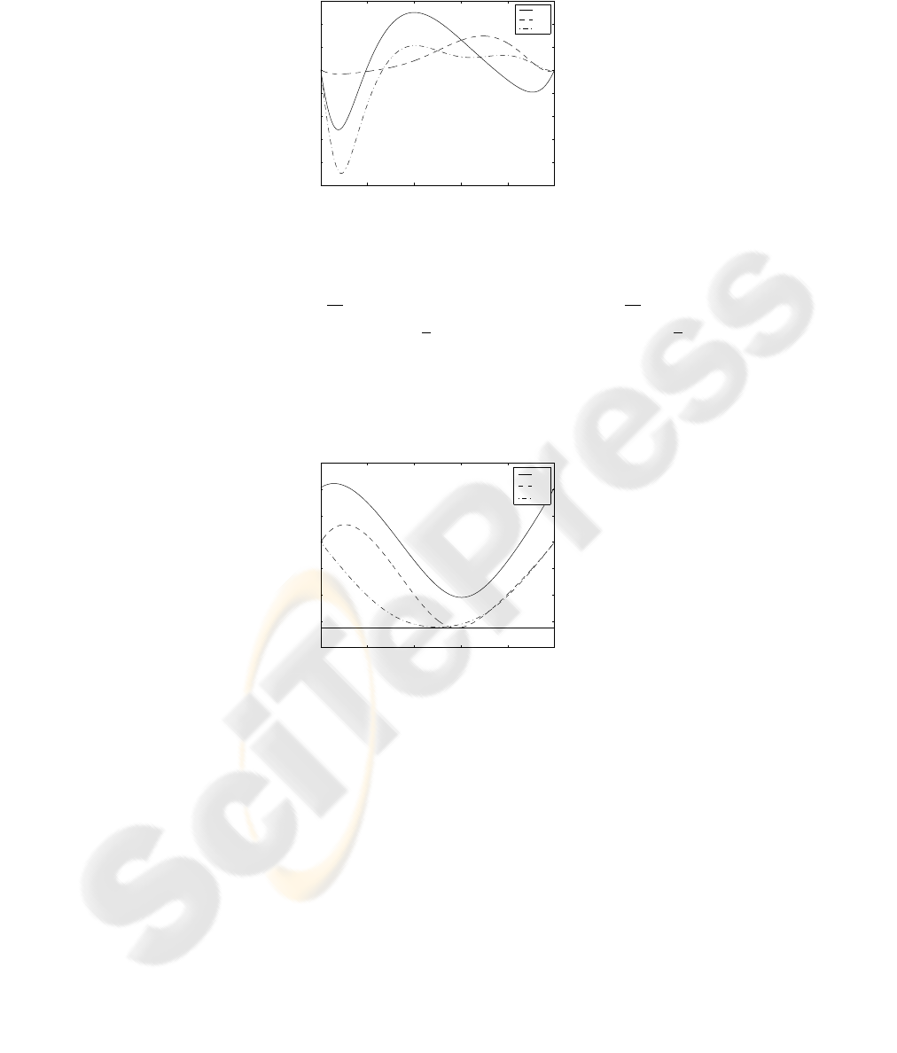
0 0.2 0.4 0.6 0.8 1
0.6
0.8
1
1.2
1.4
1.6
1.8
2
2.2
λ
v
1
, v
2
, v
3
v1
v2
v3
Fig.3. The velocities of avoiding robots R
1
, R
2
and R
3
in normalized time variable.
R
2
starts in q
s2
=
1, 0, −
3π
4
T
and has the goal pose q
g 2
=
0, 1,
3π
4
T
. The third
robot R
3
has the start pose q
s3
=
0, 0, −
π
4
T
and the goal pose q
g 3
=
1, 1,
π
4
T
. The
x and y coordinates are defined in meters. The safety distance is defined as d
s
= 0.35m.
The parameter d, which is used to define the control points P
1i
and P
2i
, equals 0.4m
(min
ij
D
ij
= 1m, γ = 0.4). In Fig. 4 the distances between the mobile robots are
0 0.2 0.4 0.6 0.8 1
0.2
0.4
0.6
0.8
1
1.2
1.4
1.6
λ
r
12
, r
13
, r
23
r
12
r
13
r
23
Fig.4. The distances between avoiding robots R
1
, R
2
and R
3
.
shown. It is also shown that all the distances r
12
, r
13
and r
23
satisfy the safety-distance
condition. They are always bigger than prescribed safety distance d
s
.
7 Conclusion
The optimal cooperative collision-avoidance approach based on B
´
ezier curves allows
us to include different criteria in the penalty functions. In our case the reference path of
each robot from the start pose to the goal pose is obtained by minimizing the penalty
function, which takes into account the sum of all the paths subjected to the distances

between the robots, which should be bigger than the minimal distance defined as the
safety distance. Current approach as presented does not include explicit velocity and
acceleration constraints to be imposed to each robot, this remaining the future research
work.
References
1. R.C. Arkin, Cooperation without communication: multiagent schema-based robot naviga-
tion, J Robot Syst., 1992, 9, 351–364,
2. L. Shan and T. Hasegawa, Space reasoning from action observation for motion planning of
multiple robots: mutal collision avoidance in a narrow passage, J Robot Soc Japan, 1996, 14,
1003–1009.
3. C.G. Kim and M.M.Triverdi, A neuro-fuzzy controller for mobile robot navigation and mul-
tirobot convoying, IEEE Trans Sys Man Cybernet SMC Part-B, 1998, 28, 829–840.
4. I. Kolmanovsky and N. H. McClamroch, Developments in Nonholonomic Control Problems,
IEEE Control Systems, 1995, 15, 6, 20–36.
5. N. Sarkar, X. Yun and V. Kumar, Control of mechanical systems with rolling constraints: Ap-
plication to dynamic control of mobile robot, The International Journal of Robotic Research,
1994, 13, 1, 55–69.
6. G. Oriolo, A. Luca and M. Vandittelli, WMR Control Via Dynamic Feedback Lineariza-
tion: Design, Implementation, and Experimental Validation, IEEE Transactions on Control
Systems Technology, 2002, 10, 6, 835–852.
7. C. Canudas de Wit and O. J. Sordalen, Exponential Stabilization of Mobile Robots with
Nonholonomic Constraints, IEEE Transactions on Automatic Control, 1992, 37, 11, 1791–
1797.
8. A. Luca, G. Oriolo and M. Vendittelli, Control of wheeled mobile robots: An experimental
overview, RAMSETE - Articulated and Mobile Robotics for Services and Technologies,
2001, S. Nicosia, B.Siciliano, A. Bicchi, P. Valigi, Springer-Verlag.
9. Y. Kanayama, Y. Kimura, F. Miyazaki and T. Noguchi, A stable tracking control method
for an autonomous mobile robot, Proceedings of the 1990 IEEE International Conference on
Robotics and Automation, 1990, 1, 384–389.
10. F. Pourboghrat and M. P. Karlsson, Adaptive control of dynamic mobile robots with non-
holonomic constraints, Computers and electrical Engineering, 2002, 28, 241–253.
11. T. C. Lee, K. T. Song, C. H. Lee and C. C. Teng, Tracking control of unicycle-modeled
mobile robots using a saturation feedback controller, IEEE Transactions on Control Systems
Technology, 2001, 9, 2, 305–318.
12. R. W. Brockett, Asymptotic stability and feedback stabilization, Differential Geometric Con-
trol Theory, 1983, R. W. Brockett, R.S. Millman and H. J. Sussmann, 181–191.
