
A LOCAL LEARNING APPROACH TO REAL-TIME
PARAMETER ESTIMATION
Application to an Aircraft
Lilian Ronceray, Matthieu Jeanneau
Stability and Control Department, Airbus France, Toulouse, France
Daniel Alazard
Philippe Mouyon
D
´
epartement Commande des Syst
`
emes et Dynamique du Vol, ONERA, Toulouse, France
Sihem Tebbani
D
´
epartement Automatique,
´
Ecole Sup
´
erieure d’
´
Electricit
´
e, Gif-sur-Yvette, France
Keywords:
Local learning, radial-basis neural networks, real-time parameter estimation.
Abstract:
This paper proposes an approach based upon local learning techniques and real-time parameter estimation, to
tune an aircraft sideslip estimator using radial-basis neural networks, during a flight test. After a presentation
of the context, we recall the local model approach to radial-basis networks. The application to the estimation
of the sideslip angle of an aircraft, is then described and the various results and analyses are detailled at the
end before suggesting some improvement directions.
1 INTRODUCTION
In the aeronautical field, although most of the useful
parameters (like inertial data, airspeed) are calculated
directly using probes, it is often relevant to use esti-
mators to consolidate the information, thus increasing
the redundancy of the aircraft systems or to replace
the probes in order to save weight. It then becomes
critical to have these estimators tuned in the early days
of the flight tests of a new aircraft, when it is only
known by an inaccurate numerical model.
The problem that is dealt with in this paper, is that
of retuning a specific estimator in real-time (or near
real-time) using flight test data. We must then take
into account that during flight tests, the aircraft flies
around in small regions of the flight domain, yielding
a strong locality constraint on the retuning.
The general idea will be to make a combined use
of local learning and real-time parameter estimation
techniques to tune the estimator, in a small neighbour-
ing of its input space, without degrading its perfor-
mance in other regions.
2 ABOUT NEURAL NETWORKS
In this section, some generalities about RBF networks
are recalled.
2.1 General Description
Such a network is composed by a set of N local es-
timators {
b
f
i
(x)}
N
i=1
, defined in the neighbouring of
some points
{
c
i
}
N
i=1
in an input space
I (Murray-
Smith, 1994).
The resulting global estimation
b
ξ is the weighted
sum of the outputs of all local estimators, for a query
point x ∈ I (see equation 1).
The weighting ϕ
i
of the local estimation
b
f
i
(x) is a
function of
k
x−c
i
k
σ
i
for all i = 1. . . N. ϕ
i
is then consid-
ered as a radial-basis function. The resulting output is
then:
b
ξ =
N
∑
i=1
ϕ
i
b
f
i
(x) (
1)
399
Ronceray L., Jeanneau M., Alazard D., Mouyon P. and Tebbani S. (2007).
A LOCAL LEARNING APPROACH TO REAL-TIME PARAMETER ESTIMATION - Application to an Aircraft.
In Proceedings of the Fourth International Conference on Informatics in Control, Automation and Robotics, pages 399-403
DOI: 10.5220/0001635103990403
Copyright
c
SciTePress

2.2 Local Parameters Computation
The local models
b
f
i
(x) can either be constants in the
neighbouring of the centers, or affine models in the
inputs, or any nonlinear model.
From now on, we will show how the parameters of
the local models are computed in the particular case
where these models are linear in the inputs (Haykin,
1999):
b
f
i
(x) = x
T
θ
i
∀x ∈
I
The problem to solve is set as follows: given a
set of K different points
{
x
k
∈ R
m
0
}
K
k=1
and a cor-
responding set of K reference values to estimate
{
ξ
k
∈ R
}
K
k=1
, find a function
b
ξ such that :
b
ξ(x
k
) = ξ
k
, ∀k = 1. . . K (2)
The RBF technique consists in choosing a func-
tion
b
ξ that has the following form :
b
ξ(x) =
N
∑
i=1
ϕ
i
x
T
b
θ
i
=
N
∑
i=1
ψ
i
(x)
T
b
θ
i
(3)
= ψ(x)
T
b
θ (4)
where N is the chosen number of local estimators, and
with ψ
i
= ϕ
i
x.
With Ψ =
{
Ψ
ki
}
=
{
ψ
i
(x
k
)
}
, the interpolation
condition (2) can be written as a linear system :
Ψ
T
b
θ = ξ (5)
In order to find a solution to equation (5) and as
Ψ is not a square matrix, we must verify that ΨΨ
T
is
nonsingular, which can be done using Michelli’s the-
orem (Michelli, 1986). A solution
b
θ satisfying the
interpolation condition (2), can then be found using
least square optimization :
b
θ
∗
=
ΨΨ
T
−1
Ψξ (6)
2.3 Selection of the Centers
A simple solution is to make a regular gridding on the
normalized input space. As minimum and maximum
variations of the input parameters are known, the in-
put space can be normalized. The gridding is then
made on a unitary hypercube.
The issue is that we face the curse of dimension-
ality though the dimension of each network’s input
space is smaller than 5. However, some physical con-
siderations, depending on the considered application,
may help reducing the number of neurons by making
a “truncated” hypercube.
For instance, in our application, some parameters
have a dependency in Mach number and angle of at-
tack α. As the aircraft is not designed to fly at both
high Mach and high α, we may remove the corre-
sponding part of the domain.
3 APPLICATION
The application we considered here is the estimation
of the sideslip angle β of a civilian aircraft, which is
the angle between the aircraft longitudinal axis and
the direction of flight (Russell, 1996).
To do so, we have a formula for the estimation
of β, based on equation (7) that describes the air-
craft lateral force equation where we neglect the lon-
gitudinal coupling terms and equation (8) which is a
classical decomposition of the lateral force coefficient
(Boiffier, 1998):
mg·Ny
cg
= P
d
SCy−F
eng,y
(7)
Cy = Cy
β
β+ ∆Cy
NL
β
+
l
V
tas
Cy
r
r+ Cy
p
p
+∆Cy
δr
+ ∆Cy
δp
(8)
where Ny
cg
denotes the lateral load factor, P
d
the
dynamic pressure, F
eng,y
the projection of thrust on
the lateral axis, β the sideslip angle, p the rolle rate,
r the yaw rate, δp the ailerons deflection, δr the rud-
der deflection, Cy
⋆
the Cy gradient w.r.t. ⋆ (β, p or r),
∆Cy
⋆
the Cy effect due to ⋆ (δp, δr or β), l the mean
aerodynamic chord andV
tas
the true airspeed velocity.
An approximation of the aircraft sideslip can then
be deduced :
b
β = −
"
1
Cy
β
#
Mg
P
d
S
Ny
cg
−
"
∆Cy
δp
Cy
β
#
−
"
∆Cy
δr
Cy
β
#
−δ
HL
"
∆Cy
NL
β
Cy
β
#
−
l
V
tas
"
Cy
p
Cy
β
#
p+
"
Cy
r
Cy
β
#
r
The key points treated in the sequel are the defi-
nition of the architecture and the initialisation of the
neural networks from a given set of simulated data,
and the in-flight tuning of these networks.
3.1 Rbf Networks Applied to Sideslip
Estimation
We will start by noticing that the expression (9) is lin-
ear in ratios of aerodynamic coefficients.
In order to ease the reader’s effort, the following
notations are introduced. Let M denote the number of
unknown ratios of aerodynamic coefficients,
b
ξ
m
the
ICINCO 2007 - International Conference on Informatics in Control, Automation and Robotics
400
m-th unknown ratio with m = 1. . . M and y
m
its at-
tached auxiliary measurement. (9) will then be writ-
ten as:
b
β =
M
∑
m=1
y
m
·
b
ξ
m
(9)
The m-th unknown ratio is modelled by a RBF net-
work with N
m
linear local estimators
b
f
i,m
(x). Its input
space
I
m
is a subset of the flight enveloppe variables.
The
b
ξ
m
depends on the following variables : α,
Mach number, P
d
, δr and δp, the last two being only
used respectively for ∆Cy
δr
and ∆Cy
δp
.
According to equation (3), estimated sideslip can
then be rewritten as :
b
β =
M
∑
m=1
y
m
ψ
m
T
b
θ
m
=
M
∑
m=1
ζ
m
T
b
θ
m
= ζ
T
Θ (10)
A linear expression of the estimated sideslip is
thus obtained, allowing the recursive least algorithm
(RLS) algorithm to be directly applied. For a com-
plete formulation of the RLS algorithm and the re-
lated criterion, one may refer to (Labarr
`
ere et al.,
1993).
3.2 The Process in Details
The process will be divided into three main parts.
Initialization: the optimal network structure must
be found : RBF, distance function, feature scaling
(transformation on the input space), centers location,
and smoothing parameter σ
i
(Atkeson et al., 1997).
A direct offline learning: where each network is
trained individually on a database of aerodynamic co-
efficient values, computed by the numerical model.
A particular attention will be paid to the norm of the
local parameter vector, which is an indicator of the
generalization performance of the network.
An indirect online learning: where the learning
criterion is no longer the error of the networks out-
puts but the error between the estimated sideslip and
the true sideslip. All the networks are trained at the
same time and must achieve both local performance,
i.e. on the considered flight point and global perfor-
mance, i.e. on the whole flight domain.
3.3 Analysis
The structure of the neural networks is a key element
in the outcome of the process and requires an analysis
of the networks’ offline performance, with respect to
the various degrees of freedom available for the net-
works’ structure.
For clarity reasons, we will only show the perfor-
mance of the (∆Cy
δr
) network in the sequel.
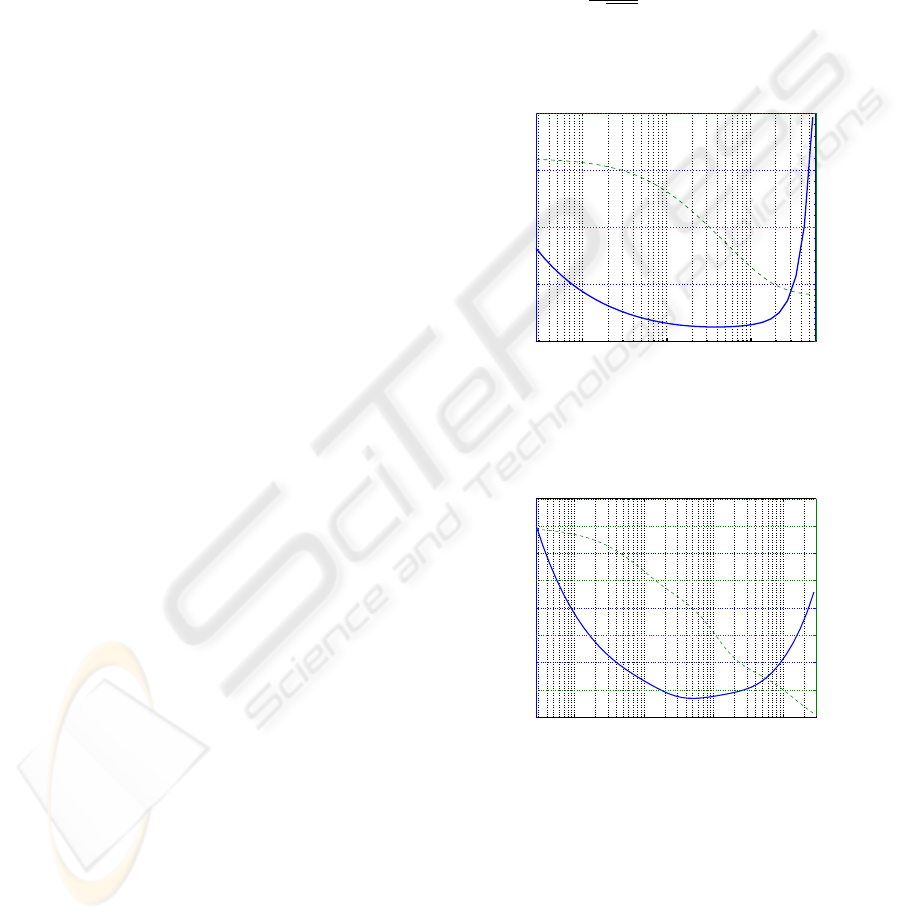
Prior to the analysis, the input space of the net-
work is normalized.The effect of the smoothing pa-
rameter σ on the learning performance and the Eu-
clidean norm of the parameter vector, which gives an
idea of the network’s capacity to generalize, will be
studied. Both the Euclidean and Infinity norm will be
used as distance functions and inverse multiquadrics
as RBF (f : x 7→
1
√
x
2
+1
). We perform an offline learn-
ing for each value of σ and compute the relative error
on the whole training data :
10
−2
10
−1
10
0
0
1000
3000
kΘk
2
σ
10
−2
10
−1
10
0
10
11
12
Relative error in %
Figure 1: Influence of σ using
k
.
k
2
.
10
−2
10
−1
10
0
10
1
0
40
80
120
160
kΘk
2
σ
10
−2
10
−1
10
0
10
1
11.6
12
12.4
12.8
Relative error in %
Figure 2: Influence of σ using
k
.
k
∞
.
The plain line represents the norm of the parame-
ter vector and the dashed line the relative error.
For both norms, we can see a behaviour that can
be compared with the overfitting phenomenon with
multilayer perceptrons (Haykin, 1999; Dreyfus et al.,
2004). We could name this “over-covering”, as it
seems that local models are strongly interfering with
each other, hence over-compensating their interac-
tion. σ must then be chosen that reaches a compro-
A LOCAL LEARNING APPROACH TO REAL-TIME PARAMETER ESTIMATION - Application to an Aircraft
401
mise between a decent performance and a relatively
small norm for the parameter vector.
In terms of compared performance, the Infin-
ity norm allows better generalization, as the norm
reaches lower values for a quite similar performance.
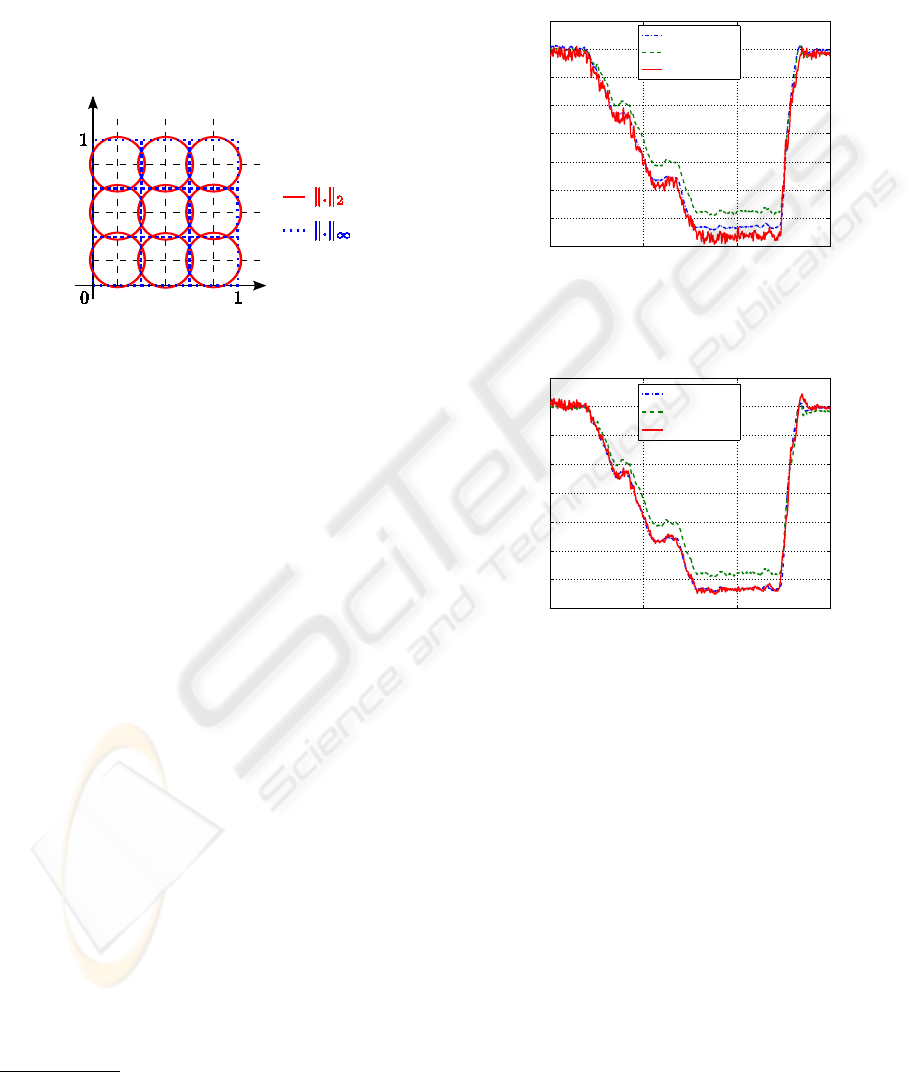
This can be justified by figure 3: the covering of 2D
normalized space is presented using gaussian kernels
with Euclidean (solid line circles) and Infinity norm
(dotted lines squares).
Figure 3: Input space covering using
k
.
k
2
and
k
.
k
∞
.
3.4 Implementation
We then chose the structure of our networks : linear
local models, inverse multiquadrics as RBF
1
, optimal
smoothing parameter according to the previous analy-
sis, normalisation of the input space as feature scaling
and a regular gridding to locate the centers.
To test our method, we used flight tests recordings
to be as close as possible to real conditions.
3.5 Results
The obtained results are presented in this section,
from learning on the pre-flight test identification data
to the online tuning during simulated flight tests (in-
flight recorded data is fed through the estimator).
About the offline part, as it is basic least squares
optimization, we will only say that the points were
generated randomly using an inaccurate numerical
model of the aircraft.
For the online adaptation, we will present results
in clean configuration for two distinct flight points
(FP1 and FP2) on a steady sideslip maneuver.
First, estimations without and then with the RLS
algorithm are presented. The dot-dashed line rep-
resents the real sideslip at the center of gravity,
the dashed line the estimated sideslip computed by
1
They are better suited for an implementation on an em-
bedded computer
the current method and the solid line the estimated
sideslip computed by our estimator (figures 4 and 5).
The aim is to compare the performance of the ex-
isting sideslip estimator which uses interpolated ap-
proximate values for the aerodynamic coefficients.
0 50 100 150
−7
−6
−5
−4
−3
−2
−1
0
1
time (s)
Sideslip (deg)
BETA
LBEST
BETAESTF
Figure 4: Flight point 1 - Fixed estimator.
0 50 100 150
−7
−6
−5
−4
−3
−2
−1
0
1
time (s)
Sideslip (deg)
BETA
LBEST
BETAESTF
Figure 5: Flight point 1 - RLS estimator.
The results are quite satisfactory because better
estimation than the existing estimator is achieved.
The noise we can see on both figures comes from the
Ny sensor and the derivation p and r.
The issue is the generalization and is emphasized
by the following procedure. The estimator is tuned on
FP1 then on FP2. Local performance is achieved for
both flight points as shown in figure 5 for FP1. The
estimator is then verified on FP1. We can see on fig-
ure 6 that the original performance has been degraded.
The learning algorithm does not tune locally enough
and impacts the whole flight domain.
ICINCO 2007 - International Conference on Informatics in Control, Automation and Robotics
402

0 50 100 150
−7
−6
−5
−4
−3
−2
−1
0
1
time (s)
Sideslip (deg)
BETA
LBEST
BETAESTF
Figure 6: Generalization from FP2 to FP1.
4 CONCLUSION
Throughout this paper, we studied the application of
RBF-based neural networks on the estimation of an
aircraft sideslip and tried to find a method to tune it in
real-time during a simulated flight test.
Though such networks have interesting local
properties, some improvements are required on the
different steps of the process, mainly on the gener-
alization performance. Work is currently on-going
about using total least squares algorithm instead of
the classical least squares (Huffel and Vandewalle,
1991; Bj
¨
orck, 1996) and their recursive form (Boley
and Sutherland, 1993). Other work directions will be
investigated :
• allowing directional forgetting in the RLS algo-
rithm (Kulhavy and K
´
arny, 1984)
• reducing numerical complexity
• adaptive filtering on the estimator output to soften
input noise effects
REFERENCES
Atkeson, C., Moore, A., and Schaal, S. (1997). Locally
weighted learning. AI Review, 11:11–73.
Bj
¨
orck, A. (1996). Numerical Methods for Least Squares
Problems. S.I.A.M., first edition.
Boiffier, J.-L. (1998). The Dynamics of Flight, The Equa-
tions. Wiley.
Boley, D. L. and Sutherland, K. T. (1993). Recursive total
least squares: An alternative to the discrete kalman
filter. Technical Report TR 93-32, Computer Science
Dpt, University of Minnesota.
Dreyfus, G., Martinez, J.-M., Samuelides, M., Gordon, M.,
Badran, F., Thiria, S., and H
´
erault, L. (2004). R
´
eseaux
de neurones, m
´
ethodologies et applications. Eyrolles,
second edition.
Haykin, S. (1999). Neural Networks, a comprehensive foun-
dation. Prentice-Hall, second edition.
Huffel, S. V. and Vandewalle, J. (1991). The Total Least
Squares Problem : Computational Aspects and Anal-
ysis. S.I.A.M., first edition.
Kulhavy, R. and K
´
arny, M. (1984). Tracking of slowly vary-
ing parameters by directional forgetting. Preprints of
the 9th IFAC World Congress, X:78–83.
Labarr
`
ere, M., Krief, J.-P., and Gimonet, B. (1993). Le Fil-
trage et ses Applications. C
´
epadu
`
es.
Michelli, C. A. (1986). Interpolation of scattered data :
Distance matrices and conditionally positive definite
functions. Constructive Approximation, 2:11–22.
Murray-Smith, R. (1994). Local model networks and local
learning. In Fuzzy-Duisburg, Duisburg.
Russell, J. B. (1996). Performance and Stability of Aircraft.
Arnold.
A LOCAL LEARNING APPROACH TO REAL-TIME PARAMETER ESTIMATION - Application to an Aircraft
403
