
Noisy Image Processing Using the Independent
Component Analysis Algorithm AMUSE
Salua Nassabay
1
, Ingo R. Keck
1
, Carlos G. Puntonet
1
, Juan M. G
´
orriz
2
J. P
´
erez de Inestroaa
2
and Rub
´
en M. Clemente
3
1
Department of Architecture and Technology of Computers
Universidad Granada, ETSII, 18071 Granada, Spain
2
Department of Signals and Communication
Universidad Granada, Granada, Spain
3
Department of Signals and Communication
Universidad Sevilla, Sevilla, Spain
Abstract. In this article we investigate the performance of the ICA algorithm
AMUSE when applied to images contaminated by noise. The classes of noise
we are using have gaussian, multiplicative and impulsive distributions. We find
that AMUSE copes surprisingly well with the different types of noise, including
multiplicative noise.
1 Introduction
Currently signal processing and especially the processing of images are gaining more
and more importance every day. To date, different investigations have been carried out
in the field of image processing whose results were compared to the Human Visual
System (HVS) [1], [2], [3], to model it’s capacities to adept quickly to the hugh amount
of data it is constantly receiving. In order to extract the desired information from these
images multistep procedures are necessary. In the first steps, the data is transformed
such that its underlying structure becomes visible. The obtained data is then subject
to further analysis tools in order to detect elementary components like, e.g., borders,
regions, textures etc. Finally, applications are developed which aim at solving the actual
problems like, e.g. recognition tasks or 3D reconstruction, etc. [4].
The present article is structured as follows: Section 2 offers a brief review of Inde-
pendent Componentes Analysis (ICA) and of its most important characteristics which
are exploited in Blind Source Separation (BSS). Also a brief introduction to the algo-
rithm AMUSE (Algorithm for Multiple Unknown Signals Extraction) is given. Section
3 evaluates the performance of the algorithm when applied to data of noisy images.
1.1 Relation between ICA and Images
In the left part of figure 1 the 256 x 256 pixel image “Lena” is displayed which we
have analyzed by ICA in order to obtain its typical characteristics or filters. As can be
Nassabay S., R. Keck I., G. Puntonet C., M. Górriz J., Pérez de Inestroaa J. and M. Clemente R. (2007).
Noisy Image Processing Using the Independent Component Analysis Algorithm AMUSE.
In Proceedings of the 3rd International Workshop on Artificial Neural Networks and Intelligent Information Processing, pages 83-90
DOI: 10.5220/0001635400830090
Copyright
c
SciTePress
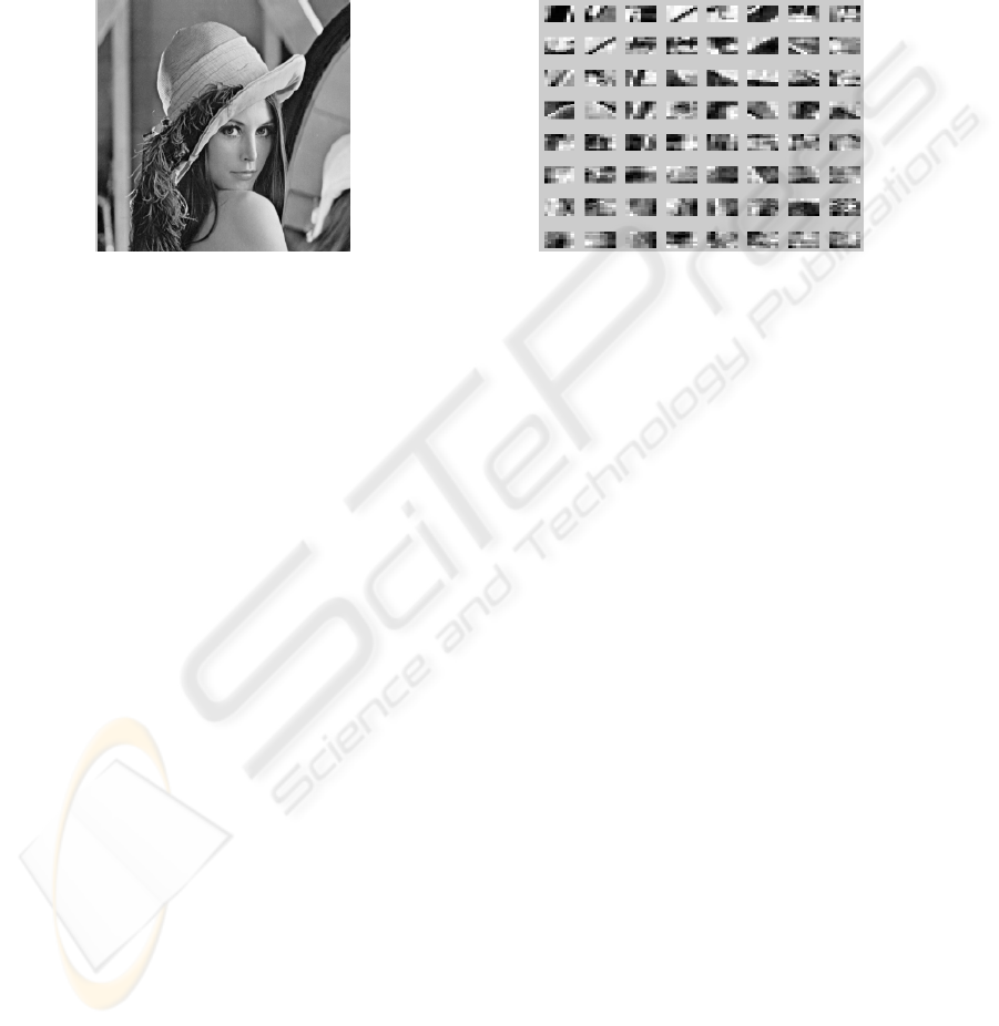
seen in the right part of Fig. 1 these characteristics exhibit edges and other structures of
interest. The characteristics were obtained by whitening the data first and by estimating
afterwards the mixing-matrix A by means of the fastICA algorithm. The shown patches
in the right part of Fig. 1 correspond to the columns a
I
of the obtained mixing matrix
A [5].
Fig. 1. Left: original image “Lena”, 256 x 256 pixels. Right: Typical characteristics of the image,
obtained applying ICA to blocks of 8 x 8 pixels.
For the processing of the image data two different approaches are usually used. The
first alternative is like a local solution where the whitening-matrix V
ZCA
= E{xx
T
}
−1/2
is used to identically filter certain local regions of the data, a procedure which is similar
to that occuring in the receptive fields in the retina and the lateral geniculate nucleus
(LGN). As second alternative Principal Component Analysis (PCA) can applied, so
that orthogonal filters are produced that lead to uncorrelated sources. Here V
PCA
=
D
−1/2
E
T
where EDE
T
= E{xx
T
} is an eigen-system of the correlation-matrix E{
ˆ
x
ˆ
x
T
}.
In addition PCA allows to reduce to the dimension of the problem by only selecting a
subgroup of the components z = V
PCA
x, which allows us, among other things, to reduce
computational costs and execution time and to lower memory consumption, etc.
Once the data has been whitened, ICA (Independent Component Analysis) is used to
find the separation- or demixing-matrix W such that the statistical dependence between
the considered sources is minimal:
ˆ
s = Wz = WV
PCA
x = WD
−1/2
n
D
T
n
x (1)
where D
n
is a diagonal matrix that contains n eigenvalues of the correlation matrix
E{xx
T
} and E
n
is the matrix having the corresponding eigenvectors in its columns.
It is important to note the similarities between the characteristics or filters found by
ICA and the receptive fields of the neurons in the primary visual cortex, a similarity
which eventually leads to the suggestion that the neurons are able to carry out a certain
type of independent component analysis and that the receptive fields are optimized for
natural images [5] [6] [7] [8].
84

2 Independent Component Analysis (ICA)
The concept of Independent Component Analysis was introduced by Heroult, Jutten and
Ans [9] as an extension of principal component analysis. The latter is a mathematical
technique that allows to project a data set to a space of characteristics whose orthogonal
basis is determined such that the variance of the projections of the data onto this basis
is larger than that obtained by projecting onto any other orthogonal basis. The resulting
signals of a PCA transform are uncorrelated which means that the covariance or the
second order cumulants, respectively, are zero.
The signals resulting from an ICA are statistically independent while no assump-
tions on the orthogonality of the basis vectors are made. The goal of such an ICA is then
to discover a new group of meaningful signals. In order to carry out this study three hy-
pothesis are necessary: the sources are mutually statistically independent; at most one
of them has a Gaussian distribution; and the mixing model (linear, convolutive or non-
linear) is known a priori. [9]
A lineal mixture x
1
,x
2
,...,x
n
of n independent components [10], [11], is expressed
mathematically by:
x
j
= a
j1
s
1
+ a
j2
s
2
+ a
j3
s
3
+ a
jn
s
n
for all j (2)
where each x
j
represents a mixture and each s
k
represents one of the independent com-
ponents. These are random variables with zero mean.
This relation can also be expressed in matrix notation: Let x be the random vector
having the mixtures x
1
,x
2
,...,x
n
as its elements, and let s be the random vector consiting
of the individual sources s
1
,s
2
,...,s
n
. Furthermore, consider the matrix A with elements
a
i j
. Following this notation the linear mixture model can be expressed as
x = As (3)
The ICA model is a generative model, where the observed data originates from a
mixture process of the hidden original components, which are mutually independent
and cannot be observed directly. This means, that only the observed data is used to
recover the mixing matrix A and the underlying sources s.
2.1 AMUSE Algorithm
The AMUSE algorithm (Algorithm for Multiple Unknown Signals Extraction) uses
temporal structures (the sources have to be uncorrelated and must have autocorrela-
tion; no assumptions on statistical independence are necessary); it applies second order
statistics with the purpose of obtaining independent components. The major motivation
for the development of this algorithm was to surpass the difficulties many fourth order
algorithms have when they are applied to problems with more than only one Gaussian
source. [12].
The AMUSE algorithm can be formulated as follows:
1. Let x(t) be whitened and let C
x
τ
have n nondegenerated eigenvalues.
85
2. The eigenvalue decomposition of C
x
τ
is determined:
C
x
τ
= W
T
DW (4)
whereas W ∈ O(n) and D is diagonal.
3. Then W is the separation matrix:
W
T
= W
−1
∼ A (5)
However, the condition that all n eigenvalues are different is often strict and are a
problem in real-life applications. The eigenvalues of Cov(s
i
(t),s
i
(T − τ )) must differ
significantly from each other, which is specially problematic with signals that have
similar energy spectra.
3 Behavior of AMUSE when Applied to Noisy Image Data
In this section we investigate the behavior of the algorithm AMUSE when applied to
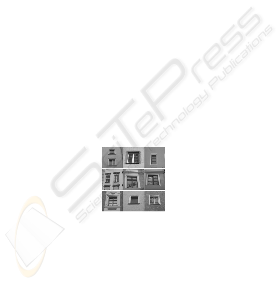
the the images shown in the figure 2.
3.1 Method
As can be seen the set of images represent structures (mostly windows) which are
displayed as grayscale pictures. These images consists of 256 × 256 pixels and each
of them was previously contaminated by Gaussian, multiplicative and impulsive (also
known as salt and pepper) noise. These types of noise can be seen as an own character-
istic function on which the following studies have been based.
Fig. 2. Some images of structures used for the analysis.
Once having contaminated the original images with each type of noise the original
and the noisy images were used to constitute the rows of the observation matrix X, i.e.
X consisted of 64 rows and 15360 columns. For them the results have been evaluated
by means of the behaviour of the filters of the different mixing matrices A as well as by
the typical distributions that must be preserved under the presence of noise.
86

Figure 3 depicts the general evaluation scheme that was used throughout this sec-
tion. First, the images of the matrix S (see figure 3) are used and transformed into the
matrix X. To these data the noise is added. From it four different observation matrices
are obtained: the observation matrix of the original mixtures (X
orig
), the observation
matrix contaminated with Gaussian noise X
gau
, the observation matrix contaminated
with multiplicative noise (X
mul
) and the observation matrix contaminated with salt and
pepper noise (X
syp
). Once the observations are created AMUSE is applied. Then the
histograms are evaluated and the different results are compared with the goal to detect
the filters which contain only noise.
Fig. 3. General diagram. Scheme that describes the separate steps of the analysis.
3.2 Behavior of AMUSE
The results obtained from this analysis are comperatively extensive as 5 different algo-
rithms and 3 classes of noise were used; its because of this reason that the algorithm
AMUSE was used at this point of the study as it exhibits a series of particularities, es-
pecially in the context of impulsive noise. Apart from this, AMUSE was found stable
no matter of the class of noise used in the data set.
First, the behavior of the bases of the mixing-matrix are investigated for each of
the two cases (original and noisy signals) after dimension reduction by PCA. In this
process the dimensions have been reduced to 49, 36, 25, 16, and 9 respectively. The
results obtained after reducing the dimension are shown in 4 for the original signals, in
5 for the signals with Gaussion noise, in 6 for signals with multiplicative noise and in 7
for signals with salt and pepper noise.
Consider for example image 4 which presents a comparison between each of the
filters while reducing the dimension, the purpose being to detect those filters which are
stable and to find out if there could be a connection between the different classes of
data. Independent of the class of noise, AMUSE found stable results in the filters, in
where each iteration of the comparison between the different dimensional reductions
also presented a concentration of stable filters in first 8 positions and mostly also in the
last 3 or 4 filters. In these figures, the red frames show the stable filters (first and last)
that stay throughout each reduction of dimension, arriving to obtain finally a reduction
87
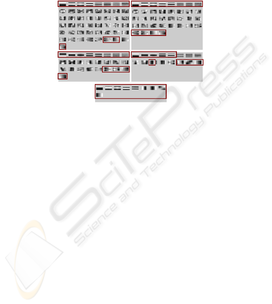
to 9 dimensions in that the filters appear clean from noise and clearly describe important
information.
Fig. 4. Results of applying AMUSE with previous PCA to the original signals. Left superior part:
reduction of dimensions to 49; right superior part: reduction of dimensions to 36; left central part:
reduction of dimensions to 25; right central part: reduction of dimensions to 16; and inferior part:
reduction of dimensions to 9.
4 Conclusion
In this article we have shown an analysis of the ICA algorithm AMUSE in digital im-
ages processing with noise. ICA has shown properties that allow to have a good model
of the characteristics of the receivers of the cortical neurons in the human visual sys-
tem. Here we have demonstrated the advantages of the ICA algorithm AMUSE that
should allow investigators to choose the best algorithm according to the necessities and
objectives that they have to consider.
Acknowledgements
The authors would like to thank Dr. Kurt Stadlthanner from the University of Regens-
burg for his help with the manuscript. This work was supported in part by the project
TEC 2004-0696 (SESIBONN).
88
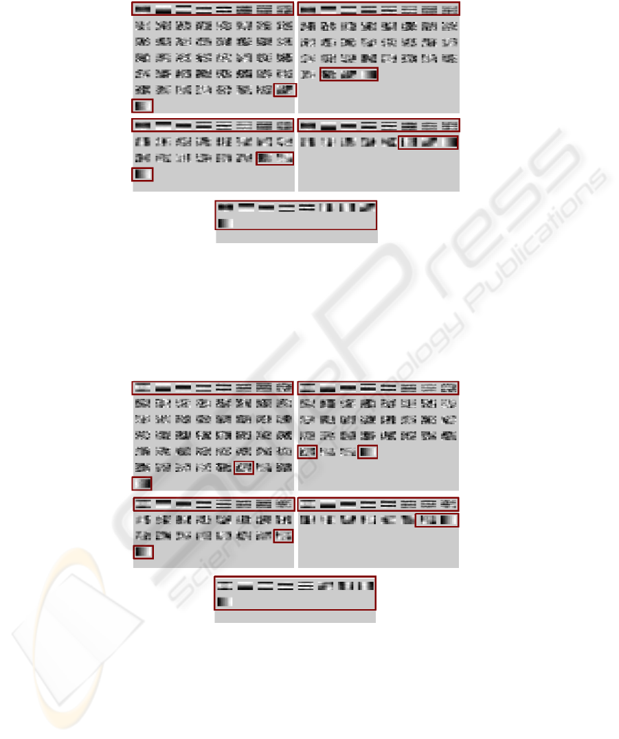
Fig. 5. Results of applying AMUSE with previous PCA to signals with gaussian noise. Left su-
perior part: reduction of dimensions to 49; right superior part: reduction of dimensions to 36; left
central part: reduction of dimensions to 25; right central part: reduction of dimensions to 16; and
inferior part: reduction of dimensions to 9.
Fig. 6. Results of applying algorithm AMUSE with previous PCA to signals with multiplica-
tive noise. Left superior part: reduction of dimensions to 49; right superior part: reduction of
dimensions to 36; left central part: reduction of dimensions to 25; right central part: reduction of
dimensions to 16; and inferior part: reduction o f dimensions to 9.
89
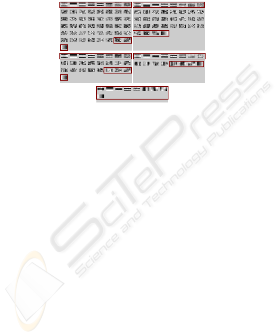
Fig. 7. Results of applying algorithm AMUSE with previous PCA to signals with salt and pep-
per noise. Left superior part: reduction of dimensions to 49; right superior part: reduction of
dimensions to 36; left central part: reduction of dimensions to 25; right central part: reduction of
dimensions to 16; and inferior part: reduction o f dimensions to 9.
References
1. Hyv
¨
arinen, A.: Sparse code shrinkage: Denoising of nongaussian data by maximum likeli-
hood estimation. In: Neural Computation. (1999) 1739–1768
2. Hyv
¨
arinen, A., Hoyer, P., Oja, E.: Imagen denoising by sparse code shrinkage. In: Intelligent
Signal Processing. (2001)
3. Pajares Martin Sanz, G., De la Cruz Garc
´
ıa, J.: Visi
´
on por computador. Im
´
agenes digitales y
aplicaciones. RA-MA Editorial Madrid. (2001)
4. Vhalupa, J.S.: The Visual Neurosciences. Werner editors. MIT Press (2003)
5. Hyv
¨
arinen, A., Karhunen, J., Oja, E.: Independent Component Analysis. Wiley Inter-science
(2001)
6. Olshausen, B.A., Field, D.J.: Emergence of simple-cell receptive field properties by learning
a sparse code for natural images. nature. In: Vision Research. (1996) 381:607–609
7. Olshausen, B.A., Field, D.J.: Sparse coding with an overcomplete basis set: A strategy
employed by v1? In: Vision Research. (1997) 37:3311–3325
8. Bell, A., Sejnowski, T.: The independent component of natural scenes are adge filters. In:
Vision Research. (1997) 3327–3338
9. H
´
erault, J., Jutten, C., Ans, B.: Detection de grandeurs primitives dans un message com-
posite par une architecture de calcul neuromimetique en apprentissage non supervise. In: X
Colloque GRETSI. (1985) 1017–10 22
10. Jutten, C., Herault, J.: Blind separation of sources, part i: An adaptive algorithm based on
neuromimetic architecture. In: Signal Processing. (1991) 24:1–10
11. Comon, P.: Independent component analysis - a new concept. In: Signal Processing. (1994)
36:287–314
12. Tong, L., Soon, V., Huang, Y., Liu, R.: Amuse: a new blind identification algorithm. In:
Circuits and Systems, IEEE International Sym posium on. Volume vol.3. (1990) 1784–1787
90
