
Robustness Against Deception in Unmanned Vehicle
Decision Making
William M. McEneaney
1
and Rajdeep Singh
2
1
Depts. of Mechanical/Aerospace Engineering and Mathematics
University of California at San Diego, La Jolla, CA 92093-0112, USA
Research partially supported by DARPA Contract NBCHC040168. and AFOSR Grant
FA9550-06-1-0238
2
Integrated Systems & Solutions, Information Assurance Group, Lockheed-Martin
La Jolla, CA, USA
Abstract. We are motivated by the tasking problem for UAVs in an adversarial
environment. In particular, we consider the problem where, in addition to purely
random noise in the observation process, the opponent may be applying decep-
tion as a means to cause us to make poor tasking choices. The standard approach
would be to apply the feedback-optimal controls for the fully-observed game, to
a maximum-likelihood state estimate. We find that such an approach is highly
suboptimal. A second approach is through a concept taken from risk-sensitive
control. For the third approach, we formulate and solve the problem directly as
a partially-observed stochastic game. A chief problem with such a formulation
is that the information state for the player with imperfect information is a func-
tion over the space of probability distributions (a function over a simplex), and
so infinite-dimensional. However, under certain conditions, we find that the infor-
mation state is finite-dimensional. Computational tractability is greatly enhanced.
A simple example is considered, and the three approaches are compared. We find
that the third approach is yields the best results (for such a case), although com-
putational complexity may lead to use of the second approach on larger problems.
1 Introduction
For a discrete deterministic game, one can apply dynamic programming techniques to
compute the value function (and “optimal” controls), defined over the state space. For
discrete stochastic games, the value function is defined over the space of all possible
probability distributions over the state space. Consequently, the problem is much more
computationally intensive. Finally, for discrete stochastic games with imperfect obser-
vations, the problem is yet more complex, and even simple games and their information
state formats become quite difficult to analyze.
We will be concerned here with a specific class of discrete stochastic games under
imperfect observations. The choice of this class will be affected by both the intended
application and computational feasibility considerations. The motivational application
here is the military command and control (C
2
) problem for air operations, with un-
manned/uninhabited air vehicles (UAVs). See [2], [5], [16], [21], [28], [31], [24], [25]
M. McEneaney W. and Singh R. (2007).
Robustness Against Deception in Unmanned Vehicle Decision Making.
In Proceedings of the 3rd International Workshop on Multi-Agent Robotic Systems, pages 74-83
Copyright
c
SciTePress

for related information. This application has specific characteristics such that we will
be able to construct a reasonable problem formulation which is particularly nice from
the point of view of analysis and computation.
We first outline the mathematical machinery. The details of the development are
discussed elsewhere due to paper length issues. After discussion of the algorithms, we
apply the techniques on a seemingly simple problem in order to determine their effec-
tiveness. We refer to the players in the game as Blue and Red, where the Blue player
has imperfect observations. We compare three Blue approaches on this simple game
problem. The most naive is for Blue to simply take the maximum likelihood estimate
of the Red state, and to apply a feedback control at this system state. As one can eas-
ily imagine, this approach is open to exploitation by Red deception. The second Blue
approach will apply a heuristic derived from the theory of Risk-Sensitive Control. This
technique is more cautious in its use of observational data. The third Blue approach (a
deception-robust approach) is through the direct solution of the imperfect information
stochastic game. As one would expect, there is an improvement in outcome with the
risk-sensitive and deception-robust approaches described herein when compared with
the standard maximum likelihood/certainty equivalence approach (although there is a
critical parameter in the risk-sensitive approach). On the other hand, there are signifi-
cant computational requirements when using these new approaches.
2 Modeling the Game
We model the state dynamics as a discrete-time Markov chain. The state will take values
in a finite set, X . Time will be denoted by t ∈ {0, 1, 2, . . . , T }. We will consider only
the problem where there are exactly two players. Blue controls will take values in a
finite set, U, and Red controls will take values in a finite set, W . Given Blue and Red
controls, and a system state, there are probabilities of transitioning to other possible
states. We let P
i,j
(u, w) denote the probability of transitioning from state i to state j in
one time step given that the Blue and Red controls are u ∈ U and w ∈ W , respectively.
Also, P (u, w) will denote the matrix of such transition probabilities. We must allow for
feedback controls. That is, the control may be state-dependent. For technical reasons,
we will find that we specifically need to consider Red feedback controls. Suppose the
size of X is n, i.e. that there are n possible states of the system. Then we may represent
a Red feedback control as w ∈ W
n
, an n-dimensional vector with components having
values in W . Specifically, w
i
= ¯w ∈ W implies that Red plays ¯w if the state is i.
Define matrix
e
P (u, w) by
e
P
i.j
(u, w) = P
i,j
(u, w
i
) ∀ i, j ∈ X . (1)
Let ξ
t
denote the (stochastic) system state at time t. Let q
t
be the vector of length n
whose i
th
component is the probability that the state is i at time t, that is the probability
that ξ
t
= i. Then if Blue plays u and Red plays w, the probability propagates as
q
t+1
=
e
P
′
(u, w)q
t
. (2)
We suppose there is a terminal cost for the game which is incurred at terminal time,
T . Let the cost for being in terminal state ξ
T
= i ∈ X be E(i), which we will also

sometimes find convenient to represent as the i
th
component of a vector, E (where we
note the abuse of notation due to use of E for two different objects). Suppose that at time
T − 1, the state is ξ
T −1
= i
0
, and that Blue plays u
T −1
∈ U and Red plays w ∈ W
n
.
Then, the expected cost would be E[E(ξ
T
)] = q
′
T
E where q
T
=
e
P
′
(u, w)q
T −1
with
q
T −1
being 1 at i
0
and zero in all other components.
We also need to define the observation process. We suppose that Red has perfect
state knowledge, but that Blue obtains its state information through observations. Let
the observations take values y ∈ Y . We will suppose that this observation process can
be influenced not only by random noise, but also by the actions of both players. For
instance, again in a military example, Blue may choose where to send sensing entities,
and Red may choose to have some entities act stealthily while having some other en-
tities exaggerate their visibility, for the purposes of deception. We let R
i
(y, u, w) be
the probability that Blue observes y given that the state is i and Blue and Red employ
controls u and w. We will also find it convenient to think of this as a vector indexed by
i ∈ X .
We suppose that at each time, t ∈ {0, 1, . . . T − 1}, first an observation occurs, and
then the dynamics occur. We let q
t
be the a priori distribution at time t, and bq
t
be the a
posteriori distribution. With this, the dynamics update of (2) is rewritten as
q
t+1
=
e
P
′
(u
t
, w
t
)bq
t
(3)
with controls u
t
, w
t
at time t. The observation, say y
t
= y, at time t updates q
t
to bq
t
via Bayes rule,
[bq
t
]
i
=
P (y
t
= y |ξ
t
= i, u, w)[q
t
]
i
P
k∈X
P (y
t
= y |ξ
t
= k, u, w)[q
t
]
k
. (4)
Then (3), (4) define the dynamics of the conditional probabilities.
2.1 Risk-Averse Controller Theory
In linear control systems with quadratic cost criteria, the control obtained through the
separation principle is optimal. That is, the optimal control is obtained from the state-
feedback control applied at the state given by
x = argmax
i
[q
t
(i)] .
A different principle, the certainty equivalence principle, is appropriate in robust con-
trol. We have applied a generalization of the controller that would emanate from this
latter principle. This generalization allows us to tune the relative importance between
the likelihood of possible states and the risk of misestimation of the state. Let us moti-
vate the proposed approach in a little more detail.
In deterministic games under partial information, the certainty equivalence principle
indicates that one should use the state-feedback optimal control corresponding to state
x = argmax [I
t
(x) + V
t
(x)] (5)
where I is the information state and V is the value function [13] (assuming uniqueness
of the argmax of course). In this problem class, the information state is essentially the

worst case cost-so-far, and the value is the minimax cost-to-come. So, heuristically, this
is roughly equivalent to taking the worst-case possibility for total cost from initial time
to terminal time. (See, for instance, [20], [17], [22], [29], [30].)
The deterministic information state is very similar to the log of the observation-
conditioned probability density in stochastic formulations for terminal/exit cost prob-
lems. In fact, this is exactly true for a class of linear/quadratic problems. In such prob-
lems, the I
t
term in (5) is replaced by the log of the probability density, and a risk-
sensitivity coefficient appears as well. Although we are outside of that problem class
here, we nonetheless apply the same approach, but where now the correct value of this
risk-sensitivity parameter is not as obvious. In particular, the risk-sensitive algorithm is
as follows: Apply state-feedback control at
x
∗
= argmax
i
{log[bq
t
(i)] + κV
t
(i)} (6)
where bq is the probability distribution based on the conditional distribution for Blue
given by (3), (4) and a stochastic model of Red control actions, and V is state-feedback
stochastic game value function (c.f. [13]). Here, κ ∈ [0, ∞) is a measure of risk aver-
sion. Note that κ = 0 implies that one is employing a maximum likelihood estimate in
the state- feedback control (for the game), i.e. argmax
i
{log([bq
t
]
i
)} = argmax
i
{[bq
t
]
i
}.
Note also (at least in linear-quadratic case where log[bq
t
]
i
= I
t
(i) modulo a constant),
κ = 1 corresponds to the deterministic game certainty equivalence principle [17], [20],
i.e. argmax{I
t
(i) + V
t
(i)}. As κ → ∞, this converges to an approach which always
assumes the worst possible state for the system when choosing a control – regardless of
observations. (See [28] for further discussion.)
2.2 Deception-Robust Controller Theory
The above approach was cautious (risk averse) when choosing the state estimate at
which to apply state-feedback control. We now consider a controller which explicitly
reasons about deception. This approach typically handles deception better that the risk-
averse approach, but this improvement comes at a substantial computational cost. For
a given, fixed computational limit, depending on the specific problem, it is not obvious
which approach will be more successful.
Here we find that the truly proper information state for Red is I
t
: Q(X ) → R,
where Q(X ) is the space of probability distributions over state space X ; Q(X ) is the
simplex in ℜ
n
such that all components are non-negative and such that the sum of
the components is one. We let the initial information state be I
0
(·) = φ(·). Here, φ
represents the initial cost to obtain and/or obfuscate initial state information. The case
where this information cannot be affected by the players may be represented by a max-
plus delta function. The information state at time t evaluated at probability distribution
q, I
t
(q), essentially represents the cost to the opponent to generate distribution q as
the naive/Bayesian distribution in a Blue estimator. That is, through obfuscation of the
initial intelligence and use of controls w
r
up to time t, the propagation (3), (4) would
lead to some q at time t if such w
r
were known. I
t
(q) would be the maximal (worst
from Blue perspective) cost to generate q by any Red controls that would yield that

particular q at time t. Although Blue does not know the Red controls, it can nonetheless
compute I
t
(·). For details on this propagation and theory, see [26].
In the case here, where the state-space is finite of size n = #X , Q is some a simplex
in IR
n
. Thus, I
t
belongs to a space of functions over an n − 1 dimensional simplex, and
consequently an element of an infinite-dimensional space. However, in the cases where
φ is either a max-plus delta function, or a piecewise-continuous function, I
t
is finite
dimensional. This is crucial to the computability of this controller. Note that in either
of these cases, the complexity of I
t
is proportional (in the worse case) to (#W )
t
at the
t time-step. Pruning strategies for reduction of this complexity are critical (c.f., [23]).
We now turn to the second component of the theory, computation of the state-
feedback value function. In this context, our value function is a generalized value func-
tion in that it is a function not only of the physical state of the system, but also of what
probability distribution Blue believes reflects its lack of knowledge of this true physical
state. The full, generalized state of the system is now described by the true state taking
values x ∈ X and the Blue conditional probability process taking values q ∈ Q(X ).
We denote the terminal cost for the game as E : X → R (where of course this does not
depend on the internal conditional probability process of Blue). Thus the state-feedback
value function at the terminal time is
V
T
(x, q) = E(x). (7)
The value function at any time, t < T , takes the form V
t
(x, q). It is he above minimax
expected payoff where Blue assumes that q is the “correct” distribution for x at time
t, that at each time Blue will know the correct q, and that Red will know both the
true physical state and this distribution, q. In particular, q will propagate according to
(2), and the state will propagate stochastically, governed by (1). Loosely speaking, this
generalized value function is the minimax expected payoff if Blue believes the state to
be distributed by q
r
at each time r ∈ (t, T ], while Red knows the true state (as well as
q
r
). A rigorous mathematical definition can be found in [26]. The backward dynamic
program that compute V
t
from V
t+1
is as follows.
1. First, let the vector-valued function M
t
be given component-wise by
[M
t
]
x
(q, u) = max
w∈W
n
h
X
j∈X
e
P
xj
(u, w)V
t+1
(j, q
′
(q, u, w))
i
(8)
where q
′
(q, u, w) =
e
P
T
(u, w) and the optimal w is
w
0
t
= w
0
t
(x, q, u) = argmax
w∈W
n
n
X
j∈X
e
P
xj
(u, w)V
t+1
(j, q
′
(q, u, w))
o
.
2. Then define L
t
as
L
t
(q, u) = q
′
M
t
(q, u), (9)
and note that the optimal u is u
0
t
(q) = argmin
u∈U
L
t
(q, u).
(10)

3. With this, one obtains the next iterate from
V
t
(x, q) =
X
j∈X
e
P
xj
(u
0
t
, w
0
t
)V
t+1
(j, q
′
(q, u
0
t
, w
0
t
)) = [M
t
]
x
(q, u
0
t
)
and the best achievable expected result from the Blue perspective is
V
1
t
(q) = q
′
M
t
(q, u
0
t
). (11)
Consequently, for each t ∈ {0, 1, . . . , T } and each x ∈ X , V
t
(x, ·) is a piecewise
constant function over simplex Q(X ). Due to this piecewise constant nature, propa-
gation is relatively straight-forward (more specifically, it is finite-dimensional in con-
tradistinction to the general case).
The remaining component of the computation of the control is now discussed. This
is typically performed via the use of the certainty equivalence principle (cf. [1], [17]),
and we employ the principle here as well. To simplify notation, note that by (9) and (8),
for any u,
L
t
(q, u) = E
q
max
w∈W
n
X
j∈X
e
P
Xj
(u, w)V
t+1
(j, q
′
(q, u, w))
.
Let us hypothesize that the optimal control for Blue is
u
m
t
.
= argmin
u∈U
max
q ∈Q(X )
{I
t
(q) + L
t
(q, u)}
. (12)
In order to obtain the robustness/certainty Equivalence result below, it is sufficient
to make the following Saddle Point Assumption. We assume that for all t,
sup
q
¯
t
∈Q
t
min
u∈U
h
I
¯
t
(q
¯
t
) + L
¯
t
(q
¯
t
, u)
i
= min
u∈U
sup
q
¯
t
∈Q
t
h
I
¯
t
(q
¯
t
) + L
¯
t
(q
¯
t
, u)
i
. (A-SP)
This type of assumption is typical in game theory. Although it is difficult to verify for a
given problem, the alternative is a theory that cannot be translated into a useful result.
Finally, after some work [26], one obtains the robustness result:
Theorem 1. Let
¯
t ∈ {0, T − 1}. Let I
0
, u
[0,
¯
t−1]
and y
[0,
¯
t−1]
be given. Let the Blue
control choice, u
m
¯
t
, given by (12) be a strict minimizer. Suppose Saddle Point Assump-
tion (A-SP) holds. Then, given any Blue strategy, λ
[
¯
t,T −1]
such that λ
¯
t
[y
·
] 6= u
m
¯
t
, there
exists ε > 0, q
ε
¯
t
and w
ε
[
¯
t,T −1]
such that
sup
q ∈Q
¯
t
{I
¯
t
(q) + L
¯
t
(q, u
m
¯
t
)} = Z
¯
t
≤ I
¯
t
(q
ε
¯
t
) + E
X∼q
ε
¯
t
n
E[E(X
ε
T
) | X
ε
¯
t
= X]
o
− ε
where X
ε
denotes the process propagated with control strategies λ
[
¯
t,T −1]
and w
ε
[
¯
t,T −1]
.
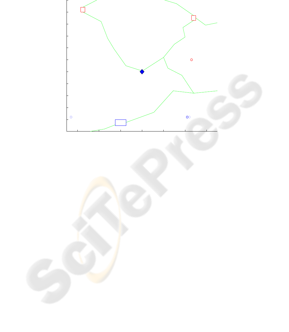
3 A Seemingly Simple Game
We now apply the above technology to an example problem in Command and Control
for UCAVs. This game will seem to be quite simple at first. However, once one intro-
duces the partial information and deception components, determination of the best (or
even nearly best) strategy becomes quite far from obvious.
−60 −40 −20 0 20 40 60
0
10
20
30
40
50
60
70
80
90
100
110
Nonlinear Example − Only one Red required to take asset
Blue base
Blue asset
Roads are in green.
Red base
Red base
number decoys on
in right group
number decoys on
in left group
number units observed
on rightnumber units observed
on left
∆
∆
∆
T
T
Fig.1. Snapshot of Gameboard.
In this game the Red player has four ground entities (say, tanks) and the Blue player
has two UCAVs. The objective of Red player is to capture the high-value Blue assets
by moving at least one non-decoy Red entity to a Blue asset location by the terminal
time, T . Red can use stealth and decoys to obscure the direction from which the attack
will occur, while the Blue player uses the UCAVs to destroy the moving Red entities.
Red entities do not have any attrition capability against the Blue UCAVs. Blue UCAVs
require at least two time steps to travel from one route to the other.
The simulation snapshot in Figure 1, is taken after time step 2, from the graphic for a
MATLAB simulation that runs the example game. Red is moving its currently surviving
three entities (depicted as triangles) downward, while Blue is attempting to prevent any
Red entities from reaching the Blue asset through use of its UCAVs (depicted as blue
T’s). Red is currently employing a decoy on the right, while using stealth on the left.
Winning and losing are measured in terms of the total cost at the terminal time. The
cost at terminal time is computed as follows: each Red surviving entitiy costs Blue 1
point and if Blue loses the high-value asset, it costs Blue 20 points.
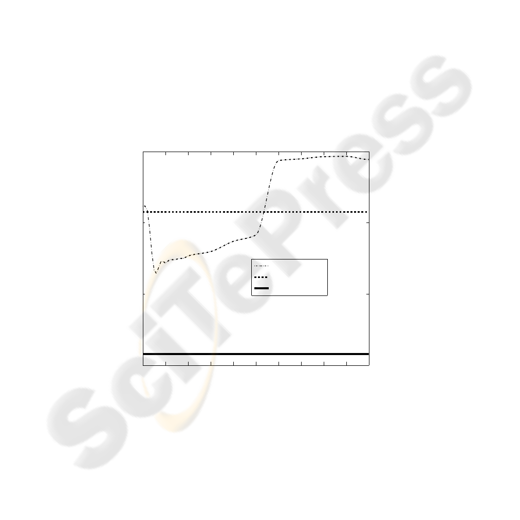
4 Comparison of the Approaches
Let us briefly foray into a comparative study between the naive approach (i.e., feed-
back on maximum-likelihood state), the risk-averse algorithm and the deception-robust
approach for Blue. The critical component of the risk-averse approach is the choice of
the risk level, κ. For the example studied in this chapter we vary κ between 0 and 10
to demonstrate the nature of the risk-averse approach in general. Firstly, for the case
κ = 0, we have the risk-averse approach equivalent to the naive approach; apply the
state-feedback control at the MLS estimate. As κ increases we expect the approach to
achieve a lower cost for Blue, since it is taking into account the expected future cost
V (X
t
) (as a risk-sensitive measure). Note however that in the adversarial environment
the effect of the Red player’s control on the Blue player’s observations has more com-
plex consequences than that of random noise. As shown in the Figure 2, the risk-averse
approach gets the best cost for Blue at κ between 0.5 and 0.6 (note again that this choice
will be problem specific). As κ increases beyond this point, the expected cost begins in-
creasing, and has a horizontal asymptote which corresponds to a Blue controller which
ignores all the observations and assumes the worst-case possible Red configuration.
0 1 2 3 4 5 6 7 8 9 10
5
10
15
20
kappa
Value
Risk−Averse
Maximum Likelihood State
Deception−robust
Comparing Different Blue Approach
Fig.2. Comparison of Approaches.
The bumpiness in the results is due to the sampling error (8000 Monte Carlo runs
were used for each data point in the plot.) Also note that for large κ, the risk-averse
approach does worse than the naive approach. For this specific example, the risk-averse

approach does not achieve the same low cost as achieved by using the deception-robust
approach.
References
1. T. Basar and P. Bernhard, H
∞
–Optimal Control and Related Minimax Design Problems,
Birkh
¨
auser (1991).
2. D.P. Bertsekas, D.A. Casta
˜
non, M. Curry and D. Logan, “Adaptive Multi-platform Schedul-
ing in a Risky Environment”, Advances in Enterprise Control Symp. Proc., (1999), DARPA–
ISO, 121–128.
3. P. Bernhard, A.-L. Colomb, G.P. Papavassilopoulos, “Rabbit and Hunter Game: Two Discrete
Stochastic Formulations”, Comput. Math. Applic., Vol. 13 (1987), 205–225.
4. T. Basar and G.J. Olsder, Dynamic Noncooperative Game Theory, Classics in Applied Math-
ematics Series, SIAM (1999), Originally pub. Academic Press (1982).
5. J.B. Cruz, M.A. Simaan, et al., “Modeling and Control of Military Operations Against Ad-
versarial Control”, Proc. 39th IEEE CDC, Sydney (2000), 2581–2586.
6. R.J. Elliott and N.J. Kalton, “The existence of value in differential games”, Memoirs of the
Amer. Math. Society, 126 (1972).
7. W.H. Fleming, “Deterministic nonlinear filtering”, Annali Scuola Normale Superiore Pisa,
Cl. Scienze Fisiche e Matematiche, Ser. IV, 25 (1997), 435–454.
8. W.H. Fleming, “The convergence problem for differential games II”, Contributions to the
Theory of Games, 5, Princeton Univ. Press (1964).
9. W.H. Fleming and W.M. McEneaney, “Robust limits of risk sensitive nonlinear filters”, Math.
Control, Signals and Systems 14 (2001), 109–142.
10. W.H. Fleming and W.M. McEneaney, “Risk sensitive control on an infinite time horizon”,
SIAM J. Control and Optim., Vol. 33, No. 6 (1995) 1881–1915.
11. W.H. Fleming and W.M. McEneaney, “Risk–sensitive control with ergodic cost criteria”,
Proceedings 31
st
IEEE Conf. on Dec. and Control, (1992).
12. W.H. Fleming and W. M. McEneaney, “Risk–sensitive optimal control and differential
games”, (Proceedings of the Stochastic Theory and Adaptive Controls Workshop) Springer
Lecture Notes in Control and Information Sciences 184, Springer–Verlag (1992).
13. W.H. Fleming and H.M. Soner, Controlled Markov Processes and Viscosity Solutions,
Springer-Verlag, New York, 1992.
14. W.H. Fleming and P.E. Souganidis, “On the existence of value functions of two–player, zero–
sum stochastic differential games”, Indiana Univ. Math. Journal, 38 (1989), 293–314.
15. A. Friedman, Differential Games, Wiley, New York, 1971.
16. D. Ghose, M. Krichman, J.L. Speyer and J.S. Shamma, “Game Theoretic Campaign Model-
ing and Analysis”, Proc. 39th IEEE CDC, Sydney (2000), 2556–2561.
17. J.W. Helton and M.R. James, Extending H
∞
Control to Nonlinear Systems: Control of Non-
linear Systems to Achieve Performance Objectives, SIAM 1999.
18. D.H. Jacobson, “Optimal stochastic linear systems with exponential criteria and their relation
to deterministic differential games”, IEEE Trans. Automat. Control, 18 (1973), 124–131.
19. M.R. James, “Asymptotic analysis of non–linear stochastic risk–sensitive control and differ-
ential games”, Math. Control Signals Systems, 5 (1992), pp. 401–417.
20. M. R. James and J. S. Baras, “Partially observed differential games, infinite dimensional HJI
equations, and nonlinear H
∞
control”, SIAM J. Control and Optim., 34 (1996), 1342–1364.
21. J. Jelinek and D. Godbole, “Model Predictive Control of Military Operations”, Proc. 39th
IEEE CDC, Sydney (2000), 2562–2567.

22. M.R. James and S. Yuliar, “A nonlinear partially observed differential game with a finite-
dimensional information state”, Systems and Control Letters, 26, (1995), 137–145.
23. W.M. McEneaney and R. Singh, “Robustness against deception”, Adversarial Reasoning:
Computational Approaches to Reading the Opponent’s Mind, Chapman and Hall/CRC, New
York (2007), 167–208.
24. W.M. McEneaney and R. Singh, “Deception in Autonomous Vehicle Decision Making in an
Adversarial Environment”, Proc. AIAA conf. on Guidance Navigation and Control, (2005).
25. W.M. McEneaney and R. Singh, “Unmanned Vehicle Operations under Imperfect Informa-
tion in an Adversarial Environment ”, Proc. AIAA conf. on Guidance Navigation and Con-
trol, (2004).
26. W.M. McEneaney, “Some Classes of Imperfect Information Finite State-Space Stochastic
Games with Finite-Dimensional Solutions”, Applied Math. and Optim., Vol. 50 (2004), 87–
118.
27. W.M. McEneaney, “A Class of Reasonably Tractable Partially Observed Discrete Stochastic
Games”, Proc. 41st IEEE CDC, Las Vegas (2002).
28. W.M. McEneaney, B.G. Fitzpatrick and I.G. Lauko, “Stochastic Game Approach to Air Op-
erations”, IEEE Trans. on Aerospace and Electronic Systems, Vol. 40 (2004), 1191–1216.
29. W.M. McEneaney, “Robust/game–theoretic methods in filtering and estimation”, First Sym-
posium on Advances in Enterprise Control, San Diego (1999), 1–9.
30. W.M. McEneaney, “Robust/H
∞
filtering for nonlinear systems”, Systems and Control Let-
ters, 33 (1998), 315–325.
31. W.M. McEneaney and K. Ito, “Stochastic Games and Inverse Lyapunov Methods in Air
Operations”, Proc. 39th IEEE CDC, Sydney (2000), 2568–2573.
32. G.J. Olsder and G.P. Papavassilopoulos, “About When to Use a Searchlight”, J. of Math.
Analysis and Applics., Vol. 136 (1988), 466–478.
33. T. Runolfsson, “Risk–sensitive control of Markov chains and differential games”, Proceed-
ings of the 32nd IEEE Conference on Decision and Control, 1993.
34. P. Whittle, “Risk–sensitive linear/quadratic/Gaussian control”, Adv. Appl. Prob., 13 (1981),
764–777.
