
CYCLE TIME OF P-TIME EVENT GRAPHS
Ph. Declerck, Ab. Guezzi and J-L. Boimond
LISA / ISTIA, University of Angers, 62 avenue Notre Dame du lac, F-49000 Angers, France
Keywords:
P-time Petri net, timed event graph, (max,+) algebra, cycle time, production rate.
Abstract:
The dater equalities constitutes an appropriate tool which allows a linear description of Timed Event Graphs in
the field of (max, +) algebra. This paper proposes an equivalent model in the usual algebra which can describe
Timed and P-time Event Graphs. Considering 1-periodic behavior, the application of a variant of Farkas’
lemma allows the determination of upper and lower bounds of the production rate and necessary conditions of
consistency.
1 INTRODUCTION
Event Graphs are a subclass of Petri nets which can
be used to model discrete event dynamic systems
subject to saturation and synchronization phenom-
ena, typically, transportation networks, multiproces-
sor systems and manufacturing systems. P-time Event
Graphs are convenient tools to model systems whose
operation times are included between a minimum
and a maximum duration. Therefore, P-time Event
Graphs can function at a maximal or a minimal speed
and, average cycle time is one of the most important
criteria which characterizes the system. An impor-
tant result about Timed Event Graphs is that a Timed
Event Graph reaches a periodic regime after a tran-
sient period (G. Cohen and Viot, 1983) (Chr
´
etienne,
1985) in the earliest functioning mode (i.e., transi-
tions fire as soon as they are enabled). In this case,
the trajectory is said K-periodic. More precisely, if
x(k) represents the date of firings of the transition x
at the number of event k, then there is a constant λ
(called the cycle time which is the inverse of the pe-
riodic throughput) and two integers k
0
in N and c in
N
∗
(called the cyclicity) such that
x(k + c) = x(k) + c × λ f or k ≥ k
0
and
λ = lim
k→∞
x(k)
k
(Gaubert, 1995).
However, the periodical behavior is reached only
after a transient that can be extremely long, moreover
presence of perturbations (faults, maintenance oper-
ations,...) can limit the possibility of reaching a pe-
riodical behavior. The representativeness of the pro-
duction rate can be reduced as the effectiveness of the
approaches as resources optimization or control using
transfert functions.
A possible approach is to generate periodic behav-
iors without transient period as 1-periodic behavior
which is defined by
x(k + 1) = x(k) + λ.
This technique assumes that each transition is struc-
turally controllable (F. Baccelli, 1992).
Considering an 1-periodic behavior, the objective
of the paper is the calculation of the average cycle
time of P-time Event Graphs. The proposed approach
introduces a new model based on ”daters” in the Sec-
tion 2. Defined by an inequality, the model com-
pletely describes in the usual algebra the trajectories
of different Event Graphs as Timed Event Graphs or
P-time Event Graphs.
Using a well-known Farkas’lemma of the linear
programming (Schijver, 1987), the Sections 3 and
4 presents results about cycle time. Two examples
are given in the Section 5 to illustrate the proposed
method.
489
Declerck P., Guezzi A. and Boimond J. (2007).
CYCLE TIME OF P-TIME EVENT GRAPHS.
In Proceedings of the Fourth International Conference on Informatics in Control, Automation and Robotics, pages 489-495
DOI: 10.5220/0001637304890495
Copyright
c
SciTePress

2 MODEL
Definition 1 A Petri net is a pair (G, M
0
), where
G = (R, V ) is a bipartite graph with a finite num-
ber of nodes (the set V ) which are partitioned into the
disjoint sets of places P and transitions T ; R consists
of pairs of the form (p
i
,q
i
) and (q
i
,p
i
) with p
i
∈ P and
q
i
∈ T . The initial marking M
0
is a vector of dimen-
sion | P | whose elements denote the number of initial
tokens in the respective places.
Definition 2 For a Petri Net with | P | places and
| T | transitions, the incidence matrix W = [W
ij
]
is an | P | × | T | matrix of integers and its typical
entry is given by W
ij
= W
+
ij
− W
−
ij
where W
+
ij
is the
weight of the arc from transition j to its output place
i and W
−
ij
is the weight of the arc to transition j from
its input place i.
In a Petri net, from a marking M , a firing sequence
implies a string of successive markings. The charac-
teristic vector s of a firing sequence S is a vector for
which each component is an integer corresponding to
the number of firings of the corresponding transition.
Then a marking M reached from M
0
by firing of a
sequence S can be deduced using the fundamental re-
lation:
M = M
0
+ W × s
where M
0
is the initial marking and W is the inci-
dence matrix.
Definition 3 A Petri net is called an Event Graph if
each place has exactly one upstream and one down-
stream transition.
P-time Petri nets allow the modeling of discrete
event dynamic systems with sojourn time constraints
of the tokens inside the places. Consistently with the
dioid
R
max
(see ((F. Baccelli, 1992))), we associate a
temporal interval defined in R
+
× (R
+
∪ {+∞}) for
each place.
Definition 4 A P-time Event Graph is a pair <
R, IS > where R is an Event Graph and the map-
ping IS: from P to R
+
× (R
+
∪ {+∞}) is defined
by p
i
→ [a
i
, b
i
] with 0 ≤ a
i
≤ b
i
.
The interval [a
i
, b
i
] is the static interval of dura-
tion time of a token in the place p
i
belonging to the
set of places P . The token must stay in the place p
i
during the minimum residence duration a
i
. Before
this duration, the token is in a state of unavailability
to fire the transition t
j
. The value b
i
is a maximum
residence duration after which the token must leave
the place p
i
(and can contribute to the enabling of the
downstream transitions). If not, the system falls into a
token-dead state. So, the token is available to fire the
transition t
j
in the time interval [a
i
, b
i
].
2.1 Preliminary Inequalities
For Event Graphs, let us express the firing interval for
each transition of the system guaranteing the absence
of token-dead states. The set
•
p is the set of input
transitions of p and p
•
is the set of output transitions
of p. The set
•
t
i
(respectively, t
•
i
) is the set of the
input (respectively, output) places of the transition t
i
.
The set of upstream (respectively, downstream) tran-
sitions of t
i
is denoted
←
t
i
=
•
(
•
t
i
) (respectively,
t
→
i
= ( t
•
i
)
•
). The following assumption alleviates
the notations. We suppose that for each pair of transi-
tions (i, j), there is at the most a unique place denoted
p
ij
between the upstream transition t
j
∈
•
p and the
downstream transition t
i
∈ p
•
. Each place p
ij
is as-
sociated with an interval [a
ij
, b
ij
], where a
ij
is the
lower bound and b
ij
the upper bound .
We consider the “dater” type well-known in the
(max, +) algebra: each variable x
i
(k) represents the
date of the k
th
firing of transition x
i
. If we assume
a FIFO functioning of the places which guarantees
that the tokens do not overtake one another, a correct
numbering of the events can be carried out. In this pa-
per, we do not take the assumption of earliest (respec-
tively, latest) functioning which will be the subject of
other studies.
Therefore, the evolution can be described by the
following inequalities expressing relations between
the firing dates of transitions. An Event Graph can be
considered as a set of subgraphs made up of a place
p
ij
linking the upstream transition j and the down-
stream transition i. We denote m
ij
the corresponding
initial marking or initial number of tokens.
For the lower bounds a
ij
of the upstream place of
transition i, we can write:
∀x
j
∈
←
x
i
, a
ij
+ x
j
(k − m
ij
) ≤ x
i
(k),
or equivalently,
x
j
(k − m
ij
) − x
i
(k) ≤ −a
ij
.
The weight 1 of x
j
(k − m
ij
) (respectively, −1
of x
i
(k)) is the weight of the entering arc of the place
p
ij
, from t
j
to place p
ij
(respectively, the outgoing arc
of the place p
ij
, from place p
ij
to transition t
i
) which
is equal to W
+
lj
(respectively, −W
−
lj
) if p
l
= p
ij
.
Respectively, for the upper bounds b
ij
of the up-
stream place of transition i, we have:
∀x
j
∈
←
x
i
, x
i
(k) ≤ b
ij
+ x
j
(k − m
ij
),
or equivalently,
x
i
(k) − x
j
(k − m
ij
) ≤ b
ij
.
The weight 1 of x
i
(k) (respectively, −1 of x
j
(k −
m
ij
)) is the weight of the entering arc of the place p
ij
,
from t
j
to place p
ij
(respectively, the outgoing arc of
the place p
ij
, from place p
ij
to transition t
i
) which is
equal to W
+
lj
(respectively, −W
−
li
) if p
l
= p
ij
.
ICINCO 2007 - International Conference on Informatics in Control, Automation and Robotics
490

2.2 Matrix Expression
Let m be the maximum number of initial tokens, the
set of the previous inequalities can be expressed as
follows:
H = [H
m
H
m−1
H
m−2
........... H
1
H
0
]×
x(k − m)
x(k − m + 1)
....
x(k − 1)
x(k)
≤
−A
B
. (1)
The matrix H contains the weights of the arcs
entering and outgoing of the places defined above.
Each place p
l
linking the upstream transition j and
the downstream transition i corresponds to two rows
of H and particularly, −A and B are vector of tem-
porizations where A
l
= a
ij
and B
l
= b
ij
.
Now, we consider the matrix representation in
different cases: the initial marking of all places is
equal to zero; the initial marking of all places is equal
to one; the general case. The two last cases will be
considered in the following sections.
a) The initial marking of all places is null
The evolution can be described by the following
inequalities expressing relations between the firing
dates of transitions:
x
j
(k) − x
i
(k) ≤ −a
ij
−x
j
(k) + x
i
(k) ≤ b
ij
.
As x(k) corresponds to firing sequence S, we can
deduce from the above description on the weight of
the arcs that there is a direct correspondance with the
incidence matrix W . Therefore, one can write the sys-
tem as follows:
H
0
× x(k) ≤
−A
B
(2)
where H
0
=
W
−W
and W = W
+
− W
−
.
b) The initial marking of all places is equal to
one
In this case, each place initially contains only one
token. One can write:
x
j
(k − 1) − x
i
(k) ≤ −a
ij
−x
j
(k − 1) + x
i
(k) ≤ b
ij
.
As x(k − 1) and x(k) respectively corresponds to
firing sequence S, we can deduce from the above de-
scription on the weight of the arcs that respectively,
there is a direct correspondance with the incidence
matrices W
+
and −W
−
. Therefore, one can write
the system as follows:
H
1
H
0
×
x(k − 1)
x(k)
≤
−A
B
with H
1
=
W
+
−W
+
and H
0
=
−W
−
W
−
.
c) General case
Now let us give the explicit form of the system (1)
or in other words, the objective is to build an equiv-
alent model such that each place of the new Event
Graph contains only zero or one token. This new form
will simplify the calculations of the cycle time.
As a place contains a maximum number of m to-
kens, the general idea is to split each place containing
m tokens into m places, where each place contains
only one token.
Let us introduce the variables α
(m−j−1)
for j = 0
to m − 1 in the inequations, we have:
x(k − m)
x(k − m + 1)
....
x(k − 3)
x(k − 2)
x(k − 1)
x(k)
=
α
(m−1)
(k − 1)
α
(m−2)
(k − 1)
....
α
(2)
(k − 1)
α
(1)
(k − 1)
α
(0)
(k − 1)
x(k)
with
α
(m−1)
(k ) = x(k − m + 1) = α
(m−2)
(k − 1)
α
(m−2)
(k ) = x(k − m + 2) = α
(m−3)
(k − 1)
.
.
.
α
(2)
(k ) = x(k − 2) = α
(1)
(k − 1)
α
(1)
(k ) = x(k − 1) = α
(0)
(k − 1)
α
(0)
(k ) = x(k)
.
Or equivalently,
α
(m−j−1)
(k) = x(k − m + j + 1) = α
(m−j−2)
(k − 1)
for j = 0 to m − 2
α
(0)
(k) = x(k)
.
The new state vector is:
X = (α
(m−1)
, α
(m−2)
, α
(m−3)
, ..., α
(2)
, α
(1)
, α
(0)
)
t
and ( 1) becomes
H
′
×
X(k − 1)
X(k)
≤
−A
B
where H
′
contains H with the addition of null
columns.
The system must be completed with 2(m − 1)× |
T | relations in the worst case: for j = 0 to m − 2,
α
(m−j−2)
(k − 1) − α
(m−j−1)
(k) ≤ 0
−α
(m−j−2)
(k − 1) + α
(m−j−1)
(k) ≤ 0
.
Therefore, one can write the system as follows:
CYCLE TIME OF P-TIME EVENT GRAPHS
491

G
1
G
0
×
X(k − 1)
X(k)
≤
0
0
with G
1
=
G
11
−G
11
and G
0
=
−G
21
G
21
.
The matrix G
11
of dimension ((m − 1)× | T | ×
m) as G
21
, is an subdiagonal of identity matrices im-
mediately above the main diagonal, while the matrix
G
21
is a diagonal of identity matrices.
Finally, we can write the algebraic form:
G
H
′
×
X(k − 1)
X(k)
≤
0
0
−A
B
.
3 CYCLE TIME
The aim of this part is the determination of the exis-
tence of 1-periodic trajectory in P-time Event Graphs.
Let us consider an Event Graph such that m
ij
= 0 or
1.
H ×
x(k)
x(k + 1)
≤
−A
B
withH =
H
11
H
10
H
21
H
20
(3)
The 1-periodic behavior can be defined by
x(k + 1) = λ × u + x(k) with u = (1, 1, ..., 1)
t
and
the average cycle time λ.
The following result will be useful.
Corollary 1 Farkas’ lemma (variant) Corollary 7.1.e
in (Schijver, 1987) (Hennet, 1989).
Let A be a matrix and let b a vector. Then the
system A × x ≤ b of linear inequalities has a solution
x, if and only if y × b ≥ 0 for each row vector y ≥ 0
with y × A = 0
Theorem 1 The system (3) can follow a 1-periodic
behavior for a given cycle time λ, if and only if, for
each row vector y ≥ 0 with
y ×
H
11
+ H
10
H
21
+ H
20
= 0, (4)
we have:
y ×
−A
B
y ×
H
10
H
20
× u
≥ λ (5)
if y ×
H
10
H
20
× u > 0,
y ×
−A
B
y ×
H
10
H
20
× u
≤ λ (6)
if y ×
H
10
H
20
× u < 0,
y ×
−A
B
≥ 0 (7)
if y ×
H
10
H
20
× u = 0.
Proof: We have
H
11
H
10
H
21
H
20
×
x(k)
λ × u + x(k)
≤
−A
B
i.e.,
H
11
× x(k) + H
10
× (λ × u + x(k)) ≤ −A
H
21
× x(k) + H
20
× (λ × u + x(k)) ≤ B
i.e.,
(H
11
+ H
10
) × x(k) ≤ −A − H
10
× (λ × u)
(H
21
+ H
20
) × x(k) ≤ B − H
20
× (λ × u)
or equivalently,
H
11
+ H
10
H
21
+ H
20
× x(k) ≤
−A
B
−
H
10
H
20
× λ × u.
(8)
From Farkas’ lemma, we can deduce that the sys-
tem (8) of linear inequalities has a solution x, if and
only if y×(
−A
B
−
H
10
H
20
×λ×u) ≥ 0 for each
row vector y ≥ 0 with y ×
H
11
+ H
10
H
21
+ H
20
= 0.
So, y ×
−A
B
− y ×
H
10
H
20
× (λ × u) ≥ 0
y ×
−A
B
≥ y ×
H
10
H
20
× (λ × u) = λ ×
y ×
H
10
H
20
× u.
In this relation, the product by u gives the addition
of all columns of
H
10
H
20
. From the sign of y ×
H
10
H
20
× u, the two cases (6)(5) and the relevant
necessary and sufficient conditions of existence of x
(7) for the system (8) can be deduced.
Let us note that the existence of a solution depends
on λ in the two first relations contrary to the last one.
ICINCO 2007 - International Conference on Informatics in Control, Automation and Robotics
492

4 LINKS WITH OTHER RESULTS
We assume that m
ij
= 1, which simplifies the pre-
sentation of the connections with notions of inci-
dence matrix and P-semi flows. So, H
11
= W
+
,
H
10
= −W
−
, H
21
= −H
11
and H
20
= −H
10
. The
previous theorem is now applied.
To summarize, for each row vector y ≥ 0 with
y ×
W
−W
= 0 (9)
- if y ×
−W
−
W
−
× u > 0 then
y ×
−A
B
y ×
−W
−
W
−
× u
≥ λ, (10)
- if y ×
−W
−
W
−
× u < 0 then
y ×
−A
B
y ×
−W
−
W
−
× u
≤ λ, (11)
- if y ×
−W
−
W
−
× u = 0 then
y ×
−A
B
≥ 0. (12)
Moreover, we consider particular vectors y: The
row-vector y can highlights the lower bounds of the
temporizations A which correspond to a Timed Event
Graph; The row-vector y can also highlight the upper
bounds of the temporizations B. However, they give a
rough estimate of λ which must be improved by con-
sidering the space of the orthogonal vectors y. Now,
we successively consider the upper bounds B and the
lower bounds A.
Upper bounds B
Let us consider a row-vector y such that the m
first entries are null. It can be defined by the vector
y = (y
1
, y
2
) with y
1
= 0. From (9), we deduce that
y
2
×W = 0. So, y
2
×W
−
×u ≥ 0, then
y
2
×B
y
2
×W
−
×u
≥
λ.
Lower bounds A
Let us consider a row-vector y such that the m
last entries are null. It can be defined by the vector
y = (y
1
, y
2
) with y
2
= 0. From (9), we deduce that
y
1
× W = 0. As W
−
≥ 0, y
1
× (−W
−
) × u ≤ 0,
then
y
1
× (−A)
y
1
× (−W
−
) × u
=
y
1
× A
y
1
× W
−
× u
≤ λ. (13)
Calculation of the state
Considering any non-negative row vector y, the
set of the relations defined by (11) (respectively, (10))
gives the lower bound (respectively, upper bound) of
λ
1
. Given an arbitrary cycle time λ
1
satisfying (11)
and (10), the objective is the calculation of the date of
firing of the transitions for a given k.
As H
11
= W
+
, H
10
= −W
−
, H
21
= −H
11
and
H
20
= −H
10
, from (8), x(k) must satisfy
W
−W
× x(k) ≤
−A
B
−
−W
−
W
−
×
λ
1
× u.
This inequality follows the general form A × x ≤
B which can be solved by the Fourier-Motzkin algo-
rithm.
4.1 Link with Karp’s Theorem
The following well-known result is based on circuits
(Gaubert, 1995).
Theorem 2 (Karp’s theorem)
In a strongly connected system, the minimal cycle
time can be defined by the maximum of the ratio of
the sum of the delays to the sum of tokens, for each
elementary circuit C
k
, i.e.,
minimal cycle time = max
k
(
sum of delays in C
k
sum of tokens in C
k
).
Let us now consider (13). Its numerator y
1
× A is
a sum of durations as y
1
> 0 which is the total delay
in C
k
.
Consider the denominator of (13): y
1
× W
−
× u.
As each row of W
−
contains a unique entrie
different from zero which can be associated with
the unique token of the relevant place, the right-
multiplication by u generates a column-vector v =
(1, 1, ..., 1)
t
whose dimension is m and which is the
initial marking M
0
. So, the denominator y
1
×W
−
×u
is equal to y
1
× M
0
which is the number of tokens
in C
k
at M
0
. Therefore, there is a correspondance
between (13) and the expression of the theorem of
Karp.
Strictly speaking, the Karp’s theorem can be apply
even if the behavior of the graph is not 1-periodic as
we suppose here.
4.2 Link with (Murata, 1989)
Another result can be found in ((Murata, 1989)). If
we model a Timed Petri Net which is consistent (i.e.,
∃ x > 0, W.x = 0) by assigning delay d
i
to each
place p
i
, then it can be shown that the minimal cycle
time is given by:
CYCLE TIME OF P-TIME EVENT GRAPHS
493
max
k
(
y
k
.D.W
+
.x
y
k
.M
0
)
where y
k
is the P-semi flow k and D is the diago-
nal matrix of d
i
,i = 1, 2, .., m.
So, W
+
.x = v and y
k
.D.W
+
.x = y
k
.A which is
the numerator of (13).
5 EXAMPLES
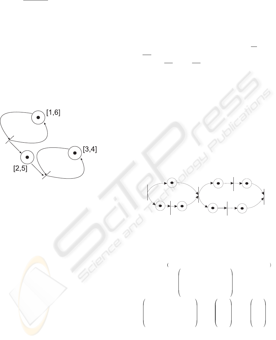
5.1 First Example
Let us consider a simple example based on two ele-
mentary strongly connected subgraphs.
Figure 1: A simple P-time Event Graph.
W
+
−W
−
−W
+
W
−
.
x(k − 1)
x(k)
≤
−A
B
with x(k) =
x
1
(k) x
2
(k) x
3
(k)
t
, W
+
=
1 0
1 0
0 1
, −W
−
=
−1 0
0 −1
0 −1
, −A =
−1
−2
−3
and B =
6
5
4
. We have
W =
0 0
1 −1
0 0
.
A possible integer matrix Y ≥ 0 such that
Y.
W
−W
= 0 is as follows. Y =
7 0 0 0 0 0
0 0 7 0 0 0
0 0 0 7 0 0
0 0 0 0 0 7
0 7 0 0 7 0
−W
−
W
−
× u =
−1 −1 −1 1 1 1
t
Y.
−W
−
W
−
× u =
−7 −7 +7 +7 0
t
Y ×
−A
B
=
−7 −21 +42 +28 +21
t
.
The two first terms lead to lower bounds (
−7
−7
= 1,
−21
−7
= 3), the two successive terms gives the upper
bounds (
+42
+7
= 6,
+28
+7
= 4) and the last one is a
condition of consistency (+21 ≥ 0).
Therefore, the 1-periodic trajectory exists with
max(1, 3) = 3 ≤ λ ≤ min(6, 4) = 4.
For λ = 3, a possible trajectory is
1
0
→
4
3
→
7
6
→ ...
For λ = 3.5, a possible trajectory is
1.5
0
→
5
3.5
→
8.5
7
→ ...
For λ = 4, a possible trajectory is
2
0
→
6
4
→
10
8
→ ...
5.2 Second Example
Now, we consider a P-time Event Graph without di-
rected circuit.
[6,8]
[4,14]
[3,5]
[2 ,11]
[0,10]
[7,9]
X
1
X
2
3
X
X
4
X
5
X
6
[1,2]
Figure 2: A P-time Event Graph.
W
+
−W
−
−W
+
W
−
.
x(k − 1)
x(k)
≤
−A
B
with x(k)
x
1
(k) x
2
(k) x
3
(k) x
4
(k) x
5
(k) x
6
(k)
t
,
W
+
=
1 0 0 0 0 0
1 0 0 0 0 0
0 0 1 0 0 0
0 1 0 0 0 0
0 1 0 0 0 0
0 0 0 1 0 0
0 0 0 0 0 1
, W
−
=
0 1 0 0 0 0
0 0 1 0 0 0
0 1 0 0 0 0
0 0 0 1 0 0
0 0 0 0 0 1
0 0 0 0 1 0
0 0 0 0 1 0
, −A =
−1
−3
−4
0
−6
−2
−7
and B =
2
5
14
10
8
11
9
W =
1 −1 0 0 0 0
1 0 −1 0 0 0
0 −1 1 0 0 0
0 1 0 −1 0 0
0 1 0 0 0 −1
0 0 0 1 −1 0
0 0 0 0 −1 1
ICINCO 2007 - International Conference on Informatics in Control, Automation and Robotics
494

A possible integer matrix Y ≥ 0 such
thatY.
W
−W
= 0 is as follows. Y =
1 0 0 0 0 0 0 1 0 0 0 0 0 0
0 1 0 0 0 0 0 0 1 0 0 0 0 0
0 0 1 0 0 0 0 0 0 1 0 0 0 0
0 0 0 1 0 0 0 0 0 0 1 0 0 0
0 0 0 0 1 0 0 0 0 0 0 1 0 0
0 0 0 0 0 1 0 0 0 0 0 0 1 0
0 0 0 0 0 0 1 0 0 0 0 0 0 1
1 0 0 0 0 0 0 0 1 1 0 0 0 0
0 1 1 0 0 0 0 1 0 0 0 0 0 0
0 0 0 1 0 1 0 0 0 0 0 1 0 1
0 0 0 0 1 0 1 0 0 0 1 0 1 0
−W
−
W
−
× u =
−1 −1 −1 −1 −1 −1 −1 1 1
1 1 1 1 1
t
Y.
−W
−
W
−
× u =
0 0 0 0 0 0 0 +1 −1 0 0
t
Y ×
−A
B
=
+1 +2 +10 +10 +2 +9 +2 +18
−5 +15 +10
t
The 9
nd
term leads to the lower bound (
−5
−1
= 5),
the 8
nd
term gives the upper bound (
+18
+1
= 18) and
the last one are conditions of consistency which are
satisfied.
Therefore, the 1-periodic trajectory exists with 5≤
λ ≤ 18
For λ = 5, a possible trajec-
tory is
3 0 1 5 4 1
t
→
8 5 6 10 9 6
t
→
13 10 11 15 14 11
t
→ ...
6 CONCLUSION
Using a new incidence matrix, the model we propose
allows the counting of the events in Timed and P-time
Event Graphs. The connections with usual incidence
matrix has been realized. Considering 1-periodic be-
havior, the application of a variant of Farkas’ lemma
leads to the introduction of a generalization of the
P-semi flow vectors for Timed and P-time Event
Graphs, and allows the determination of upper and
lower bounds of the possible cycle time. Each limit
is respectively a complex function of lower and up-
per bounds of the temporizations. Moreover, even if
cycle time λ belongs to this interval, the system must
also satisfy conditions of consistency such that the fi-
nite initial dates of firing exist. With the restriction
that a 1-periodic behavior has been considered, the
proposed lower bound of the cycle time includes the
Karp’s relation.
REFERENCES
Chr
´
etienne, P. (1985). Analyse des r
´
egimes transitoire et
asymptotique d’un graphe d’
´
ev
´
enements temporis
´
e.
Technique et Science Informatique, pages 127-142.
F. Baccelli, G. Cohen, G. O. J.-P. Q. (1992). Synchroniza-
tion and Linearity: An Algebra for Discrete Event Sys-
tems. Wiley.
G. Cohen, D. Dubois, J.-P. Q. and Viot, M. (1983). Anal-
yse du comportement p
´
eriodique de syst
`
emes de pro-
duction par la th
´
eorie des dioides. In Rapport de
recherche. INRIA.
Gaubert, S. (November 1995). Resource optimization and
(min, +) spectral theory. In IEEE Transactions on Au-
tomatic Control, Vol. 40, No. 11.
Hennet, J.-C. (1989). Une extension du lemme de farkas
et son application au probl
`
eme de r
´
egulation lin
´
eaire
sous contraintes. In Compte-Rendus
`
a l’Acad
´
emie des
Sciences, t. 308, S
´
erie I, pp. 415-419.
Murata, T. (1989). Petri nets: Properties, analysis and ap-
plications. In Proceedings of the IEEE, Vol. 77, No.
4.
Schijver, A. (1987). Theory of linear and integer program-
ming. John Wiley and Sons.
CYCLE TIME OF P-TIME EVENT GRAPHS
495
