
BENCHMARKING HAAR AND HISTOGRAMS OF ORIENTED
GRADIENTS FEATURES APPLIED TO VEHICLE DETECTION
Pablo Negri, Xavier Clady and Lionel Prevost
Universit
´
e Pierre et Marie Curie-Paris 6, ISIR, CNRS FRE 2507
3 rue Galil
´
ee, 94200 Ivry sur Seine, France
Keywords:
Intelligent vehicle, vehicle detection, AdaBoost, Haar filter, Histogram of oriented gradient.
Abstract:
This paper provides a comparison between two of the most used visual descriptors (image features) nowadays
in the field of object detection. The investigated image features involved the Haar filters and the Histogram of
Oriented Gradients (HoG) applied for the on road vehicle detection. Tests are very encouraging with a average
detection of 96% on realistic on-road vehicle images.
1 INTRODUCTION
On road vehicle detection is an essential part of the In-
telligent Vehicles Systems and has many applications
including platooning (i.e. vehicles travelling in high
speed and close distances in highways), Stop&Go
(similar that precedent situation, but at low speeds),
and autonomous driving.
Most of the detecting methods distinguish two ba-
sic steps: Hypothesis Generation (HG) and Hypoth-
esis Verification (HV) (Sun et al., 2006). HG ap-
proaches are simple low level algorithm used to lo-
cate potential vehicle locations and can be classified
in three categories:
- knowledge-based: symmetry (Bensrhair et al.,
2001), colour (Xiong and Debrunner, 2004; Guo
et al., 2000), shadows (van Leeuwen and Groen,
2001), edges (Dellaert, 1997), corners (Bertozzi
et al., 1997), texture (Bucher et al., 2003), etc.,
- stereo-based: disparity map (Franke, 2000), inverse
perspective mapping (Bertozzi and Broggi, 1997),
etc,
- and motion-based (Demonceaux et al., 2004).
HV approaches perform the validation of the Re-
gions of Interest generated by the HG step. They can
be classified in two categories: template-based and
appearance-based. Template-based methods perform
a correlation between a predefined pattern of the vehi-
cle class and the input image: horizontal and vertical
edges (Srinivasa, 2002), regions, deformable patterns
(Collado et al., 2004) and rigid patterns (Yang et al.,
2001). Appearance-based methods learn the charac-
teristics of the classes vehicle and non-vehicle from
a set of training images. Each training image is rep-
resented by a set of local or global descriptors (fea-
tures) (Agarwal et al., 2004). Then, classification al-
gorithms can estimate the decision boundary between
the two classes.
One of the drawbacks of optical sensors are the
considerable time processing and the average robust-
ness. In that way, Viola & Jones (Viola and Jones,
2001) developed simple an appearance-based system
obtaining amazing results in real time. Their appear-
ance based method uses Haar-based representation,
combined with an AdaBoost algorithm (Freund and
Schapire, 1996). They also introduce the concept of
a cascade of classifiers which reaches high detection
results while reducing computation time.
The present article compares the Haar-based fea-
tures with the Histograms of Oriented Gradient (HoG)
based features using the same cascade architecture.
The next section describes briefly the Haar and
the HoG features. Section two introduces the learn-
ing classification algorithms based on AdaBoost. We
finish the article with the results and conclusions.
359
Negri P., Clady X. and Prevost L. (2007).
BENCHMARKING HAAR AND HISTOGRAMS OF ORIENTED GRADIENTS FEATURES APPLIED TO VEHICLE DETECTION.
In Proceedings of the Fourth International Conference on Informatics in Control, Automation and Robotics, pages 359-364
DOI: 10.5220/0001637503590364
Copyright
c
SciTePress
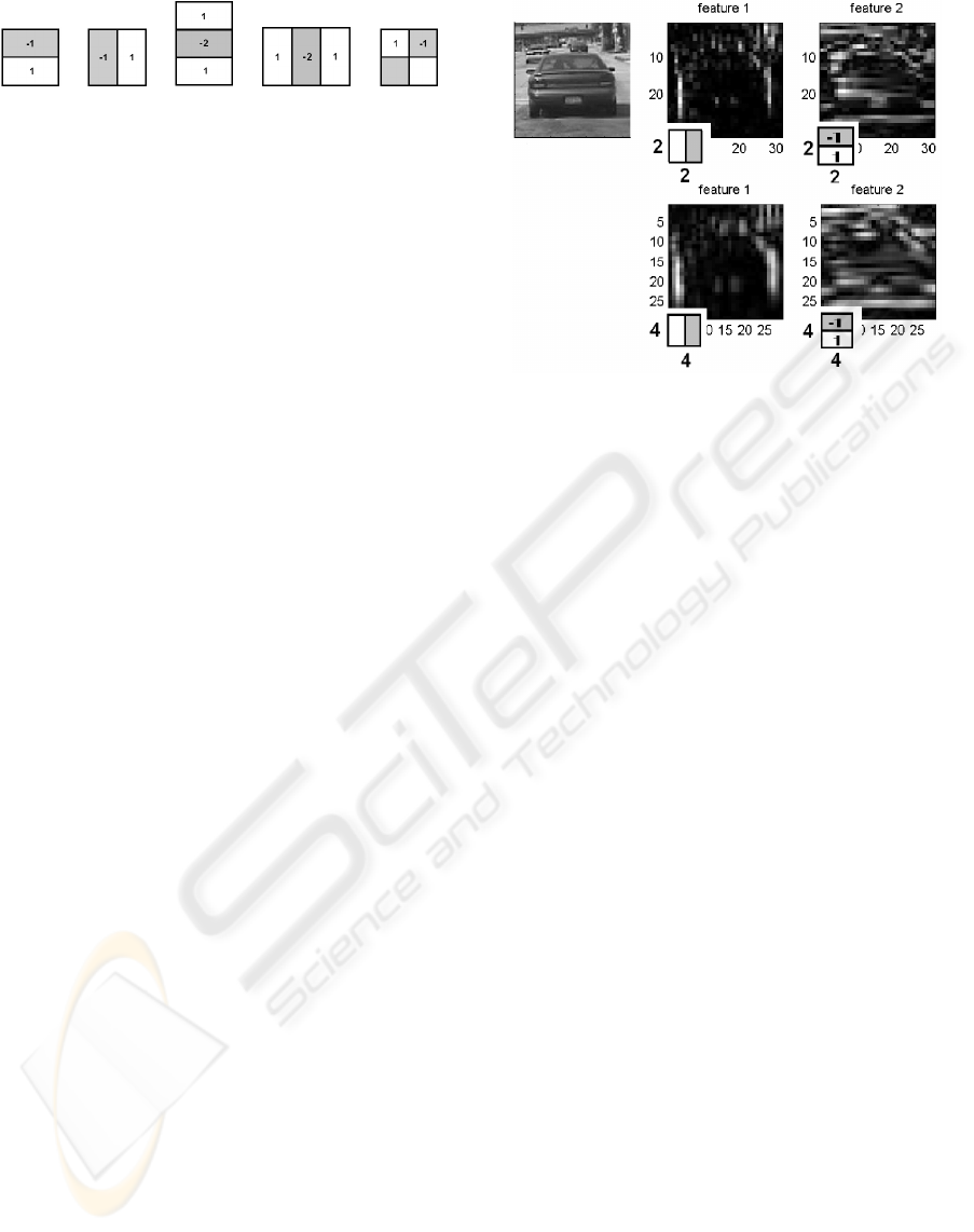
Figure 1: 2D Wavelet set.
2 FEATURES
The common reasons why features are choosen in-
stead of pixels values are that features can code high
level object information (segments, texture, ...) while
intensity pixel values based system operates slower
than a feature based system. This section describes
the features used to train the Adaboost cascade.
2.1 Haar Filters
Each wavelet coefficient describes the relationship
between the average intensities of two neigh-boring
regions. Papageorgiou et al. (Papageorgiou and
Poggio, 1999) employed an over-complete set of 2D
wavelets to detect vehicles in static images.
Figure 1 shows basic Haar filters: two, three and
four rectangle features, where the sum of the pixels
which lie within the white rectangles are subtracted
from the sum of pixels in the grey rectangles. We con-
serve the two and three rectangle features since vehi-
cles have rectangular shape: diagonal features (four
rectangle template) doesn’t give extra information for
this type of pattern.
Viola & Jones (Viola and Jones, 2001) have intro-
duced the Integral Image, an intermediate representa-
tion for the input image. The sum of the rectangular
region in the image can be calculated in four Integral
Image references. Then, the difference between two
adjacent rectangles, can be computed with only six
references, eight in the case of the three rectangle fea-
ture.
The Haar feature set is composed of the resulting
value of the rectangular filters at various scales in a
image.
In figure 2 we can see the results of two rectan-
gular filters (vertical and horizontal) at two scales:
2x2 and 4x4 pixels. Lightness pixels mean important
subtraction values (the result is always calculated in
modulus). The complete set of Haar’s features uti-
lizing the three rectangular filters (see fig. 1) in a
32x32 pixel image at {2,4,8,16} scales is 11378. Ev-
ery single feature j in the set could be defined as:
f
j
= (x
j
, y
j
, s
j
, r
j
), where r
j
is the rectangular filter
type, s
j
the scale and (x
j
, y
j
) are the position over the
32x32 image.
Figure 2: 2D Haar Wavelet example on a vehicle image.
2.2 Histogram of Oriented Gradient
The Histograms of Oriented Gradient (HoG) is an-
other way to encode an input image to obtain a vec-
tor of visual descriptors. This local descriptor, based
on Scale Invariant Feature Transform (SIFT) (Lowe,
1999), uses the gradient magnitude and orientation
around a keypoint location to construct an histogram.
Orientations are quantized by the number of bins in
the histogram (four orientations are sufficient). For
each histogram bin, we compute the sum in the re-
gion of all the magnitudes having that particular ori-
entation. The histogram values are then normalised
by the total energy of all orientations to obtain values
between 0 and 1.
Gepperth (Gepperth et al., 2005) train a neural net-
work classifier using these features for a two class
problem: vehicle, non-vehicle. First, a ROI is sub-
divided into a fixed number of regions called recep-
tive fields. From each receptive field, they obtain an
oriented histogram feature.
The HoG features set is composed of histograms
calculated inside a rectangular region on the original
image. We evaluate the the gradient of the image us-
ing the Sobel filters to obtain the gradient magnitude
and orientation.
There are three types of rectangle regions: r
1
square l*l, r
2
vertical rectangle l*2l, r
3
horizontal
rectangle 2l*l. Considering l : {2,4, 8, 16} scales, we
have a total of 4678 features. A single histogram j in
the set could be defined as: h
j
= (x
j
, y
j
, s
j
, r
j
), where
r
j
is the rectangular filter type, s
j
the scale and (x
j
, y
j
)
are the position over the 32x32 image.
ICINCO 2007 - International Conference on Informatics in Control, Automation and Robotics
360
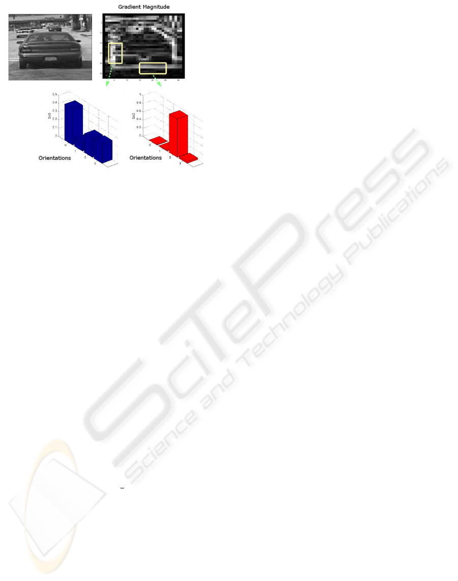
Figure 3: HoG example on a vehicle image.
3 ADABOOST
As we saw in previous sections, Haar and HoG rep-
resentations are used to obtain a vector of visual de-
scriptors describing an image. The size of these vec-
tors is clearly bigger than the number of pixel in the
image. Using the total number of features to carry
out a classification is inadequate from the computing
time point of view of the and the robustness, since
many of these features do not contain important infor-
mation (noise). Different methods: statistics (Schnei-
derman and Kanade, 2000), PCA, genetic algorithms
(Sun et al., 2004), etc. can be used to select a limited
quantity of representative features.
Among these methods, the Boosting (Freund and
Schapire, 1996) classification method improves the
performance of any algorithm. It finds precise hy-
pothesis by combining several weak classifiers which,
on average, have a moderate precision. The weak
classifiers are then combined to create a strong clas-
sifier:
G =
1
∑
N
n=1
α
n
g
n
≥
1
2
∑
N
n=1
α
n
= T
0 otherwise
(1)
Where G and g are the strong and weak classifiers
respectively, and α is a coefficient wheighting each
feature result. T is the strong classifier threshold.
Different variants of boosting are known such as
Discrete Adaboost (Viola and Jones, 2001), Real Ad-
aBoost (Friedman et al., 2000), Gentle AdaBoost, etc.
The procedures (pseudo-code) of any of this variants
are widely developed in the literature.
We need, however, to study the construction of the
weak classifier for both cases: Haar and HoG fea-
tures.
3.1 Haar Weak Classifier
We define the weak classifier as a binary function g:
g
1 if p
j
f
j
< p
j
θ
j
0 otherwise
(2)
where f
j
is the feature value, θ
j
the feature threshold
and p
j
the threshold parity.
3.2 Hog Weak Classifier
This time, instead of evaluate a feature value, we es-
timate the distance between an histogram h
j
of the
input image and a model histogram m
j
. The model
is calculated like the mean histogram between all the
training positive examples. For each histogram h
j
of
the feature set, we have the corresponding m
j
. A ve-
hicle model is then constructed and AdaBoost will
found the most representative m
j
which best separate
the vehicle class from the non-vehicle class.
We define the weak classifier like a function g:
g
1 if d(h
j
, m
j
) > θ
j
0 otherwise
(3)
where d(h
j
(x), m
j
) is the Bhattacharyya distance
(Cha and Srihari, 2002) between the feature h
j
and m
j
and θ
j
is the distance feature threshold.
4 TEST AND RESULTS
4.1 Dataset
The images used in our experiments were collected
in France using a prototype vehicle. To ensure data
variety, 557 images where captured during different
time, and on different highways.
The training set contains 745 vehicle sub-images
of typical cars, sport-utility vehicles (SUV) and mini-
van types. We duplicate this quantity flipping the sub-
images around y-axis, obtaining 1490 examples. We
split this new set keeping 1000 of the examples for
training and the others for validation: the training set
(TS) contains 1000 sub-images aligned to a resolution
of 32 by 32 pixels, the validation set (VS) contains
490 vehicle sub-images with the same resolution. The
negative examples come from 3196 images without
vehicles.
The test set contains 200 vehicles in 81 images.
4.2 Single Stage Detector
First experiments were carried out with a strong clas-
sifier constructed with 100, 150 and 200 Haar or HoG
BENCHMARKING HAAR AND HISTOGRAMS OF ORIENTED GRADIENTS FEATURES APPLIED TO VEHICLE
DETECTION
361
features using the Discrete Adaboost algorithm (Viola
and Jones, 2001).
We used the TS for the positive examples. The
non-vehicle (negatives) examples were collected by
selecting randomly 5000 sub-windows from a set of
250 non-vehicle images at different scales.
To evaluate the performance of the classifiers, the
average detection rate (DR) and the number of false
positives (FP) were recorded using a three-fold cross
validation procedure. Specifically, we obtain three
sets of non-vehicle sub-windows to train three strong
classifiers. Then, we test these classifiers on the test
set.
4.3 Multi Stage Detector
This section shows the test realised using a cascade of
strong classifiers (Viola and Jones, 2001). The multi
stage detector increases detection accuracy and re-
duces the computation time. Simpler classifiers (hav-
ing a reduced number of features) reject the majority
of the false positives before more complex classifiers
(having more features) are used to reject difficult sub-
windows.
Stages in the cascade are constructed with the Ad-
aboost algorithm, training a strong classifier which
achieves a minimum detection rate (d
min
= 0.995) and
a maximum false positive rate ( f
max
= 0.40). The
training set is composed of the TS positive examples
and the non-vehicle images separated in 12 different
folders (the maximum number of stages). Subsequent
classifiers are trained using those non-vehicle images
of the corresponding folder which pass through all the
previous stages.
An overall false positive rate is defined to stop the
cascade training process (F = 43 ∗ 10
−7
) within the
maximum number of stages.
This time, the average accuracy (AA) and false
positives (FP) where calculated using a five-fold cross
validation procedure. We obtain five detectors from
five differents TS and VS randomly obtained.
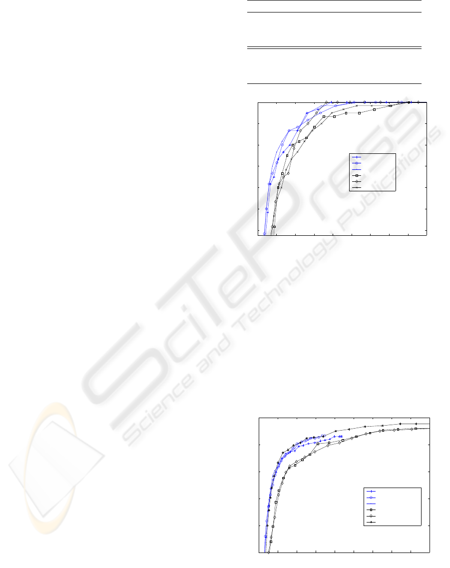
4.4 Results
Table 1 shows the detection rate of the single stage
detector trained either on Haar features or on HoG
features with respectively 100, 150 and 200 features.
These results are very interesting though quite pre-
dictible. As seen before, HoG classifiers computes
a distance from the test sample to a ”vehicle model”
(the mean histograms). These are generating classi-
fiers. When the number of considered features in-
creases, the model is refined and the detection rate in-
creases while the number of false positives keeps sta-
Table 1: Single stage detection rates (Haar and HoG classi-
fiers).
Classifier DR (%) FP Time
HoG - 100 fts 69.0 1289 3,52
HoG - 150 fts 72.5 1218 4,20
HoG - 200 fts 83.1 1228 5,02
Haar - 100 fts 96.5 1443 2,61
Haar - 150 fts 95.7 1278 3,93
Haar - 200 fts 95.8 1062 5,25
0 0.005 0.01 0.015 0.02 0.025 0.03 0.035 0.04 0.045
0.94
0.95
0.96
0.97
0.98
0.99
1
FP
AA
Haar 100 fts
Haar 150 fts
Haar 200 fts
HoG 100 fts
HoG 150 fts
HoG 200 fts
Figure 4: ROC curves for Haar and HoG Single Stage de-
tectors.
ble. On the other hand, Haar classifiers are discrimi-
native classifier evaluating a fronteer between positive
and negative samples. Now, the fronteer is refined -
and the number of false positives decreases - when
the number of features increases. Figure 4 presents
the ROC curves for each detector. As told before, for
a given detection rate, the number of false positives is
lower for Haar classifiers than for HoG classifiers.
0 0.5 1 1.5 2 2.5 3 3.5 4 4.5
x 10
−3
0.75
0.8
0.85
0.9
0.95
1
FP
AA
Haar − N = 1000
Haar − N = 2000
Haar − N = 3000
HoG − N = 1000
HoG − N = 2000
HoG − N = 3000
Figure 5: ROC curves for Haar and HoG Multi Stage detec-
tors.
ICINCO 2007 - International Conference on Informatics in Control, Automation and Robotics
362
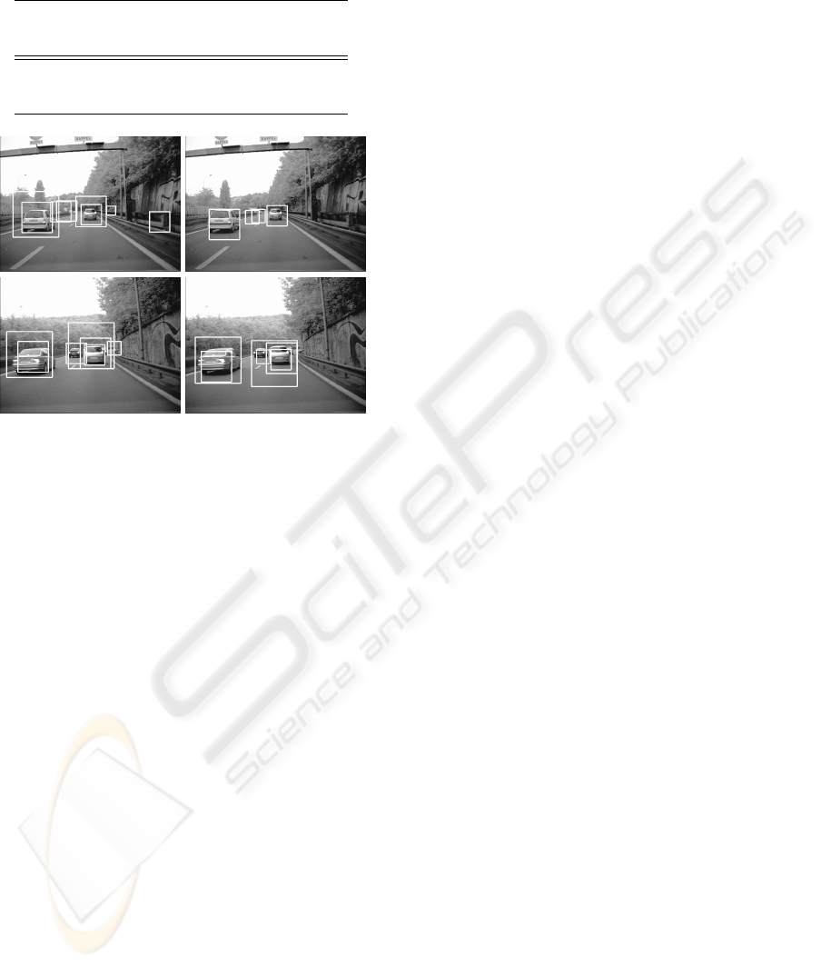
Table 2: Multi stage detection rate (Haar and HoG classi-
fiers).
Classifier Stages # Fts # Neg DR (%) FP t (seg)
Haar 12 306 1000 94.3 598 0.75
Haar 12 332 2000 94 490 0.71
Haar 12 386 3000 93,5 445 0.59
HoG 12 147 1000 96.5 935 0.51
HoG 12 176 2000 96.1 963 0.59
HoG 11 192 3000 96.6 954 0.55
(a) (b)
Figure 6: Detection results for (a) HoG and (b) Haar Multi
Stage detectors.
Table 2 shows results of cascade detectors using
Haar and HoG based features. We also tested the
effect of increasing the size of the negative set in
each training stage. The behavior of each detector is
the same as described before. HoG detector try to
construct a finer vehicle model to take into account
the new negatives. The number of features used in-
creases as the model refines. But the detection rate
and the number of false positives does not change
significantly. Haar detector refines the fronteer using
somemore features and the number of false positives
decreases while the detection keeps quite stable. Fig-
ure 5 shows the ROC curves for each detector applied
for the last stage in the cascade. For a given detection
rate, these curves show a similar behavior as the sin-
gle stage detector, where the number of false positives
is lower for the Haar classifiers than for the HoG clas-
sifiers; except for the HoG detector trained with 3000
negatives, which has a similar behavior with a half
quantity of features (see table 2). Figure 6 presents
some detection results and false alarms.
5 CONCLUSION
This communication deals with a benchmark com-
paring Haar-like features and Histograms of Oriented
Gradients features applied to vehicle detection. These
features are used in a classification algorithm based
on Adaboost. Two strategies are implemented: a sin-
gle stage detector and a multi-stage detector. The
tests - applied on realistic on-road images - show two
different results: for the HoG (generative) features,
when the number of considered features increases, the
detection rate increases while the number of false pos-
itives keeps stable; for the Haar-like (discriminative)
features, the number of false positives decreases. Fu-
ture works will be oriented to combined these behav-
iors. An approach could be build using simultane-
ously both feature types. We should also select rele-
vant features.
ACKNOWLEDGEMENTS
This research was supported by PSA Peugeot Citro
¨
en.
The authors would liko to thank Fabien Hernan-
dez from PCA Direction de la Recherche et de
l’Innovation Automobile for their help with the data
collection.
REFERENCES
Agarwal, S., Awan, A., and Roth, D. (2004). Learning to
detect objects in images via a sparse, part-based rep-
resentation. IEEE Transactions on Pattern Analysis
and Machine Intelligence, 26(11):1475–1490.
Bensrhair, A., Bertozzi, M., Broggi, A., Miche, P., Mousset,
S., and Toulminet, G. (2001). A cooperative approach
to vision-based vehicle detection. In Proceedings on
Intelligent Transportation Systems, pages 207–212.
Bertozzi, M. and Broggi, A. (1997). Vision-based vehicle
guidance. Computer, 30(7):49–55.
Bertozzi, M., Broggi, A., and Castelluccio, S. (1997). A
real-time oriented system for vehicle detection. Jour-
nal of Systems Architecture, 43(1-5):317–325.
Bucher, T., Curio, C., Edelbrunner, J., Igel, C., Kastrup,
D., Leefken, I., Lorenz, G., Steinhage, A., and von
Seelen, W. (2003). Image processing and behavior
planning for intelligent vehicles. IEEE Transactions
on Industrial Electronics, 50(1):62–75.
Cha, S. and Srihari, S. N. (2002). On measuring the
distance between histograms. Pattern Recognition,
35(6):1355–1370.
Collado, J., Hilario, C., de la Escalera, A., and Armingol, J.
(2004). Model based vehicle detection for intelligent
vehicles. In International Symposium on Intelligent
Vehicles, pages 572–577.
BENCHMARKING HAAR AND HISTOGRAMS OF ORIENTED GRADIENTS FEATURES APPLIED TO VEHICLE
DETECTION
363

Dellaert, F. (1997). Canss: A candidate selection and search
algorithm to initialize car tracking. Technical report,
Robotics Institute, Carnegie Mellon University.
Demonceaux, C., Potelle, A., and Kachi-Akkouche, D.
(2004). Obstacle detection in a road scene based
on motion analysis. IEEE Transactions on Vehicular
Technology, 53(6):1649 – 1656.
Franke, U. (2000). Real-time stereo vision for urban traf-
fic scene understanding. In Proceedings IEEE Intel-
ligent Vehicles Symposium 2000, pages 273–278, De-
troit, USA.
Freund, Y. and Schapire, R. (1996). Experiments with a
new boosting algorithm. In International Conference
on Machine Learning, pages 148–156.
Friedman, J., Hastie, T., and Tibshirani, R. (2000). Additive
logistic regression: a statistical view of boosting. The
Annals of Statistics, 28(2):337–374.
Gepperth, A., Edelbrunner, J., and Bocher, T. (2005). Real-
time detection and classification of cars in video se-
quences. In Intelligent Vehicles Symposium, pages
625–631.
Guo, D., Fraichard, T., Xie, M., and Laugier, C. (2000).
Color modeling by spherical influence field in sensing
drivingenvironment. In IEEE, editor, Intelligent Vehi-
cles Symposium, pages 249–254, Dearborn, MI, USA.
Lowe, D. (1999). Object recognition from local scale-
invariant features. In Proceedings of the International
Conference on Computer Vision, pages 1150–1157.
Papageorgiou, C. and Poggio, T. (1999). A trainable ob-
ject detection system: Car detection in static images.
Technical report, MIT AI Memo 1673 (CBCL Memo
180).
Schneiderman, H. and Kanade, T. (2000). A statistical
method for 3d object detection applied to faces and
cars. In ICCVPR, pages 746–751.
Srinivasa, N. (2002). Vision-based vehicle detection and
tracking method for forward collision warning in au-
tomobiles. In IEEE Intelligent Vehicle Symposium,
volume 2, pages 626–631.
Sun, Z., Bebis, G., and Miller, R. (2004). Object detection
using feature subset selection. Pattern Recognition,
37(11):2165–2176.
Sun, Z., Bebis, G., and Miller, R. (2006). On-road vehicle
detection: A review. IEEE Trans. Pattern Anal. Mach.
Intell., 28(5):694–711.
van Leeuwen, M. and Groen, F. (2001). Vehicle detec-
tion with a mobile camera. Technical report, Com-
puter Science Institute, University of amsterdam, The
Netherlands.
Viola, P. and Jones, M. (2001). Rapid object detection using
a boosted cascade of simple features. In Conference
on Computer Vision and Pattern Recognition, pages
511–518.
Xiong, T. and Debrunner, C. (2004). Stochastic car track-
ing with line- and color-based features. Advances
and Trends in Research and Development of Intelli-
gent Transportation Systems: An Introduction to the
Special Issue, 5(4):324–328.
Yang, H., Lou, J., Sun, H., Hu, W., and Tan, T. (2001).
Efficient and robust vehicle localization. In Interna-
tional Conference on Image Processing, volume 2,
pages 355–358, Thessaloniki, Greece.
ICINCO 2007 - International Conference on Informatics in Control, Automation and Robotics
364
