
BOUNDARY CONTROL OF A CHANNEL
Last Improvements
Val
´
erie Dos Santos
Universit
´
e de Lyon, Lyon, F-69003, France ; Universit
´
e Lyon 1, CNRS, UMR 5007, LAGEP, Villeurbanne, F-69622, France
ESCPE, Villeurbanne, F-69622, France
Christophe Prieur
LAAS-CNRS, 7 avenue du Colonel Roche, 31077 Toulouse, Cedex 4, France
Keywords:
Lyanpunov stability, Proportionnal-Integral control, Saint-Venant equations, Riemann coordinates.
Abstract:
Different improvements have been developed in regards to the stability and the control of two-by-two non
linear systems of conservation laws, and in particular for the Saint-Venant equations and the control of flow
and water level on irrigation channel. One stability result based on the Riemann coordinates is presented
here and sufficient conditions are given to insure the Cauchy convergence. Another result still based on the
Riemann approach is presented too, in the linear case, to improve the feedback control based on the Riemann
invariants.
1 INTRODUCTION
In this paper, we are concerned with the stability of
the non linear Saint-Venant equations, a two-by-two
systems of conservation laws, that are described by
hyperbolic partial differential equations, with one in-
dependent time variable t ∈ [0,∞) and one indepen-
dent space variable, x ∈ [0,L]. For such systems, the
considered boundary control problem is the problem
of designing feedback control actions at the bound-
aries (i.e. at x = 0 and x = L) in order to ensure that
the smooth solution of the Cauchy problem converge
to a desired steady state.
This problem has been previously considered in the
literature ((Litrico et al., 2005)), and in our previ-
ous papers (Coron et al., 2002). Those results have
been improved in (Dos Santos et al., 2007) in order to
take account of non homogeneous terms (like pertur-
bations, slope or frictions) adding an integral part to
the Riemann control developed.
Recently, the non linear problem of the stability of
systems of two conservation laws perturbed by non
homogeneous terms has been investigated (Prieur
et al., 2006), (Dos Santos and Prieur, 2007), using the
state evolution of the Riemann coordinates.
This paper aim is to shortly present both last results
develop on (Dos Santos and Prieur, 2007), (Dos San-
tos et al., 2007) and to illustrate them with simula-
tions and experimentations based on a river data and
the Valence micro-channel respectively.
After a short presentation of the shallow water equa-
tions, the first problem is stated, the tools presented,
and the stability result established. The second result
is developed in the same way in the fourth section and
the simulations results are produced as well as the ex-
perimentations ones in the last part.
2 DESCRIPTION OF THE
MODEL: SAINT-VENANT
EQUATIONS
We consider a reach of an open channel as represented
in Figure 1.
We assume that the channel is prismatic with a con-
stant rectangular section. Note that in our configura-
tion, the slope could be non null as well as the friction
effects.
The flow dynamics are described by a system of two
laws of conservation (Saint-Venant or shallow water
equations), namely a law of mass conservation and a
law of momentum conservation
∂
t
H + ∂
x
(Q/B) = 0, (1)
∂
t
Q+ ∂
x
(
Q
2
BH
+
1
2
gBH
2
) = gBH(I −J), (2)
320
Dos Santos V. and Prieur C. (2007).
BOUNDARY CONTROL OF A CHANNEL - Last Improvements.
In Proceedings of the Fourth International Conference on Informatics in Control, Automation and Robotics, pages 320-325
DOI: 10.5220/0001637903200325
Copyright
c
SciTePress
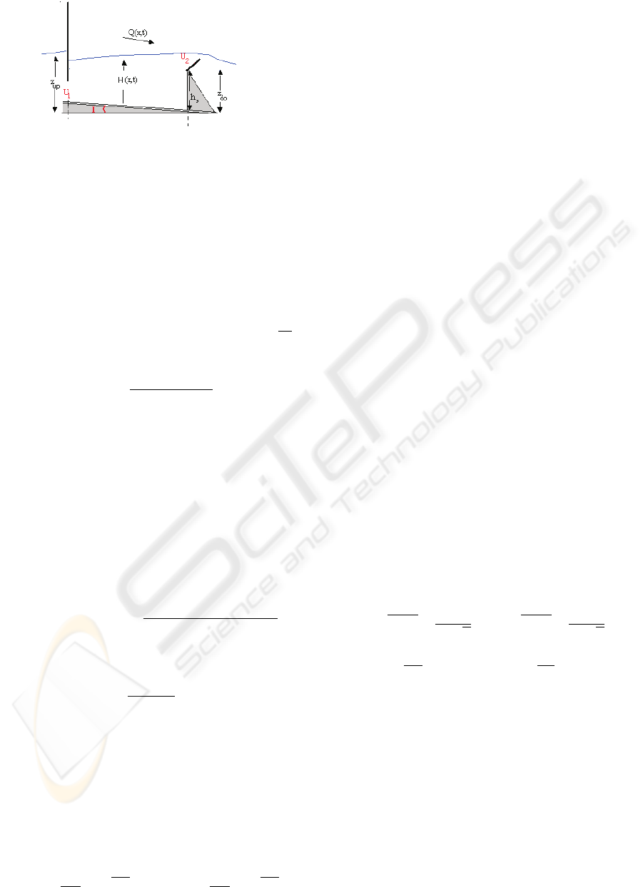
Figure 1: Scheme of a channel: one reach with an overflow
gate.
where H(t,x) stands for the water level and Q(t, x) the
water flows in the reach while g denotes the gravita-
tion constant (m.s
−2
). I is the bottom slope (m.m
−1
),
B is the channel width (m) and J is the slope’s friction
(m.m
−1
).
The slope’s friction J is expressed with the Manning-
Strickler expression, (n
M
is the Manning coefficient
(s.m
−1/3
) and the Strickler coefficient is K =
1
n
M
(m
1/3
.s
−1
)),
J(Q,H) =
n
2
M
Q
2
S(H)
2
R(H)
4/3
,
where S(H) is the wet surface (m
2
) and P(H) the wet
perimeter (m): S(H) = BH,P(H) = B+ 2H, R(H) is
the hydraulic radius (m), R(H) = S(H)/P(H).
The control actions are the positions U
0
and U
L
of the two spillways located at the extremities of the
pool and related to the state variables H and Q by the
following expressions.
Two cases may occur for the gate equations at x = 0
and x = L:
• a submerged underflow gate:
Q(x
i
,t) = U
i
Bµ
i
p
2g(H
1
(x
i
,t) −H
2
(x
i
,t)),(3)
• or a submerged overflow gate:
H
1
(x
i
,t) = (
Q
2
(x
i
,t)
2gB
2
µ
2
i
)
1/3
+ h
s,i
+U
i
, (4)
where H
1
(x,t) is the water level before the gate,
H
2
(x,t) is the water level after the gate and h
s,i
is the
height of the fixed part of the overflow gate n
◦
i (Fig.
(1)) and µ
i
is the water flow coefficient of the gate n
◦
i
located at x = x
i
.
Note that the system (1)-(2) is strictly hyperbolic,
i.e. its Jacobian matrix has two non-zero real distinct
eigenvalues:
λ
1
(H,V) =
Q
BH
+
p
gH, λ
2
(H,V) =
Q
BH
−
p
gH.
They are generally called characteristic velocities.
The flow is said to be fluvial (or subcritical) when the
characteristic velocities have opposite signs:
λ
2
(H,V) < 0 < λ
1
(H,V).
Different stability results have been given for the
linearized system (Coron et al., 2007)-(Dos Santos
et al., 2007) and the non-linear one (Prieur et al.,
2006)-(Dos Santos and Prieur, 2007) using the prop-
erties of Riemann coordinates. Those results are
quickly resumed in both following sections.
3 FIRST RESULT: INTEGRAL
ACTIONS AND LYAPUNOV
STABILITY ANALYSIS
3.1 Linearized System
An equilibrium (H
e
,Q
e
) is a constant solution of the
equations (1)-(2) , i.e. H(t,x) = H
e
, Q(t,x) = Q
e
∀t
and ∀x which satisfies the relation:
J(H
e
,Q
e
) = I. (5)
A linearized model is used to describe the variations
around this equilibrium. The following notations are
introduced:
h(t, x) ˆ=H(t, x) −H
e
(x), q(t, x) ˆ=Q(t, x) −Q
e
(x).
The linearized model around the equilibrium
(H
e
,Q
e
) is then written as
∂
t
h(t, x) + ∂
x
q(t, x) = 0 (6)
∂
t
q(t, x) + cd∂
x
h(t, x) + (c−d)∂
x
q(t, x) =
−γh(t, x) −δq(t, x), (7)
with:
c =
p
gBH
e
+
Q
e
H
e
√
B
, d =
p
gBH
e
−
Q
e
H
e
√
B
γ = gBH
e
∂J
∂H
(H
e
,Q
e
), δ = gBH
e
∂J
∂Q
(H
e
,Q
e
).
In the special case where the channel is horizontal
(I = 0) and the friction slope is negligible (n ≈0), we
observe that γ = δ = 0 and that this linearized system
is exactly in the form of the following linear hyper-
bolic system:
∂
t
h(t, x) + ∂
x
q(t, x) = 0 (8)
∂
t
q(t, x) + cd∂
x
h(t, x) + (c−d)∂
x
q(t, x) = 0. (9)
It is therefore legitimate to apply the control with
integral actions that have been analyzed in (Coron
et al., 2007) to open channels having small bottom
and friction slopes.
BOUNDARY CONTROL OF A CHANNEL - Last Improvements
321

3.2 Riemann Coordinates and Stability
Conditions
In order to solve this boundary control problem, the
Riemann coordinates (see e.g. (Renardy and Rogers,
1993) p. 79) defined by the following change of coor-
dinates are introduced :
a(t, x) = q(t,x) + dh(t, x) (10)
b(t, x) = q(t,x) −ch(t, x) (11)
With these coordinates, the system (8)-(9) is written
under the following diagonal form :
∂
t
a(t, x) + c∂
x
a(t, x) = 0 (12)
∂
t
b(t, x) −d∂
x
b(t, x) = 0 (13)
In the Riemann coordinates, the control problem can
be restated as the problem of determining the control
actions in such a way that the solutions a(t,x), b(t, x)
converge towards zero.
The boundary control laws u
0
(t) and u
L
(t) are defined
such that the boundary conditions (3)-(4) expressed
in the Riemann coordinates satisfy the linear relations
(Coron et al., 2007) augmented with appropriate inte-
grals as follows:
a
0
(t) + k
0
b
0
(t) + m
0
y
0
(t) = 0 (14)
b
L
(t) + k
L
a
L
(t) + m
L
y
L
(t) = 0 (15)
where k
0
, k
L
and m
0
, m
L
are constant design param-
eters that have to be tuned to guarantee the stability.
The integral y
0
on the flow q at the boundary x = 0
and the integral y
L
on the other state h at the bound-
ary x = L are defined as:
y
0
(t) =
t
0
q
0
(s)ds =
t
0
ca
0
(s) + db
0
(s)
c+ d
ds
y
L
(t) =
t
0
h
L
(s)ds =
t
0
a
L
(s) −b
L
(s)
c+ d
ds.
Using Lyapunov theory, one can prove this theorem:
Theorem 1 Let m
0
, m
L
and k
0
, k
L
four constants such
that the six following inequalities hold:
m
0
> 0, m
L
< 0, (16)
|k
0
| < 1, |k
0
k
L
| < 1, (17)
|k
L
| <
c
d
d
c
< 1, (18)
Then there exist five positive constants A, B, µ, N
0
and
N
L
such that, for every solution (a(t,x),b(t,x)), t > 0,
x ∈ [0,L], of (12), (13), (14) and (15) the following
function:
U(t) =
A
c
L
0
a
2
(t, x)e
−µx/c
dx+
c+ d
2
N
0
y
2
0
(t)
+
B
d
L
0
b
2
(t, x)e
µx/d
dx+
c+ d
2
N
L
y
2
L
(t)
satisfies:
˙
U ≤ −µU.
Remark 1 As it has been mentioned above, in our
previous paper (Coron et al., 2007) the special case
with m
0
= m
L
= 0 in the boundary conditions (14)-
(15) and N
0
= 0, N
L
= 0 has been treated. We have
shown that inequality |k
0
k
L
| < 1 is sufficient to have
˙
U < −µU for some µ > 0 along the system trajectories
and ensure the convergence of a(t, x) and b(t,x) to
zero.
In the fifth section, we shall illustrate the effi-
ciency of the control with simulations on a realistic
model of a waterway and with experimental results
on a real life laboratory plant.
4 SECOND RESULT: STABILITY
OF THE NON-LINEAR
SAINT-VENANT EQUATIONS
Previous result delead with the stability of two con-
servation laws systems, which can be written as (8)-
(9) (Coron et al., 2007), i.e. for homogeneous hyper-
bolic systems. The stability condition depends thus of
the spectral radius of the Jacobian matrix linked. In
(Prieur et al., 2006), those results have been extended
to the non homogeneous system, with an additional
condition on the size of the non homogeneous terms.
Here, we proposed a new result that improve the suf-
ficient stability condition |k
0
k
L
| < 1 (Dos Santos and
Prieur, 2007).
4.1 Statement
In order to introduce the problem under consideration
in this work, we need some additional notations:
• The usual euclidian norm |·| in R is denoted by
|·|. The ball centered in 0 ∈ R with radius ε > 0
is denoted B(ε);
• Given Φ continuous on [0,L] and Ψ continuously
differentiable on [0,L], we denote
|Φ|
C
0
(0,L)
= max
x∈[0,L]
|Φ(x)| ,
|Ψ|
C
1
(0,L)
= |Ψ|
C
0
(0,L)
+ |Ψ
′
|
C
0
(0,L)
;
• the set of continuously differentiable functions
Ψ
#
: [0,L] → R satisfying the compatibility as-
sumption
C and |Ψ
#
|
C
1
(0,L)
≤ ε is denoted B
C
(ε).
For constant control actions U
0
(t) =
¯
U
0
and
U
L
(t) =
¯
U
L
, a steady-state solution is a constant so-
lution (H,Q)(t, x) =
¯
H,
¯
Q
(x) for all t ∈ [0, +∞),
ICINCO 2007 - International Conference on Informatics in Control, Automation and Robotics
322

for all x ∈[0, L] which satisfies (1)-(2) and the bound-
ary conditions (3)-(4).
At time t ≥ 0, the output of the system (1)-(2) is
given by the following
y(t) = (H
0
(t), H
L
(t)) (19)
The problem under consideration in this work is
the following: Given a steady-state
¯
H,
¯
Q
T
, called
the set point, we consider the problem of the lo-
cal exponential stabilization of (1)-(2) by means of
a boundary output feedback controller, i.e. we want
to compute a boundary output feedback controller
y 7→ (U
0
(y),U
L
(y)) such that, for any smooth small
enough (in C
1
-norm) initial condition H
#
and Q
#
sat-
isfying our compatibility conditions, the PDE (1)-(2)
with the boundary conditions (3)-(4) and the initial
condition
(H, Q)(x, 0) = (H
#
,Q
#
)(x) ,∀x ∈ [0,L]. (20)
has a unique smooth solution converging exponen-
tially fast (in C
1
-norm) towards
¯
H,
¯
Q
T
.
4.2 Stability Result
First note that the system (1)-(2) is strictly hyperbolic,
i.e. the Jacobian matrix of this system has two non-
zero real distinct eigenvalues:
λ
1
(H, Q) =
Q
BH
+
p
gH, λ
2
(H, Q) =
Q
BH
−
p
gH.
They are generally called characteristic velocities.
The flow is said to be fluvial (or subcritical) when
the characteristic velocities have opposite signs:
λ
2
(H, Q) < 0 < λ
1
(H, Q).
Under constant boundary conditions Q(0,t) =
¯
Q
0
and
H(L,t) =
¯
H
L
, for all t, there exists a steady state solu-
tion x 7→(
¯
Q,
¯
H) satisfying
∂
x
¯
Q(x) = 0, ∂
x
¯
H(x) = −g
¯
H
I−
¯
J
¯
λ
1
¯
λ
2
,
(21)
with
¯
λ
1
= λ
1
(
¯
H,
¯
Q), and
¯
λ
2
= λ
2
(
¯
H,
¯
Q).
Let t
1
and t
2
be the time instants defined by
x
1
(t
1
) = L , x
2
(t
2
) = 0, (22)
where x
i
, i = 1,2, are the solution of the Cauchy prob-
lem
˙x
i
(t) = λ
i
(
¯
H,
¯
Q), x
1
(0) = 0, x
2
(L) = 0.
To state our stability result, we need to introduce
the following notations
¯a = (
¯
Q
B
¯
H
+ 2
p
g
¯
H) ,
¯
b = (
¯
Q
B
¯
H
−2
p
g
¯
H).
We can explicit functions f
1
and f
2
, and expres-
sions ℓ
1
and ℓ
2
depending on the equilibrium and on
the perturbations such that, for all i ∈ {1,2},
ℓ
i
= f
i
(
¯
λ
i
, ¯a,
¯
b,I,n
M
) . (23)
Due to space limitation, the explicit expression of ℓ
1
and ℓ
2
is omitted, it is developed in (Dos Santos and
Prieur, 2007).
The boundary conditions are written as follows:
a(t, 0) + k
0
b(t, 0) = 0 (24)
b(t, L) + k
L
a(t, L) = 0, (25)
where k
0
, k
L
are constant design parameters that have
to be tuned to guarantee the stability.
We are now in position to state our stability result,
here in the case of a reach bounded by two underflow
gates:
Theorem 2 Let t
1
, t
2
, ℓ
1
and ℓ
2
be defined by (22),
and (23) respectively.
If the bottom slope function I, the slope’s friction
function J are sufficiently small in C
1
norm, then we
have
max(t
1
ℓ
1
,t
2
ℓ
2
) < 1 , (26)
In that case, there exist k
0
and k
L
such that
| k
0
k
L
| +t
2
| k
0
| ℓ
2
+t
1
ℓ
1
< 1, (27)
| k
0
k
L
| +t
1
| k
L
| ℓ
1
+t
2
ℓ
2
< 1. (28)
The following boundary output feedback controller
U
0
= H
0
¯
Q
0
B
¯
H
0
−2
√
gα
0
√
H
0
−
p
¯
H
0
µ
0
p
2g(z
up
−H(0,t))
, (29)
U
L
= H
L
¯
Q
L
B
¯
H
L
+ 2
√
gα
L
√
H
L
−
p
¯
H
L
µ
L
p
2g(H(L,t) −z
do
)
, (30)
where H
0
= H(t,0), H
L
= H(t,L), α
0
=
1−k
0
1+k
0
, and
α
L
=
1−k
L
1+k
L
make the closed loop system locally ex-
ponentially stable, i.e. there exist ε
0
> 0, C > 0 and
µ > 0 such that, for all initial conditions (H
#
,Q
#
) :
[0,L] → (0,+∞) continuously differentiable, satisfy-
ing some compatibility conditions and the inequality
|(H
#
,Q
#
) −(
¯
H,
¯
Q)|
C
1
(0,L)
≤ ε,
there exists a unique C
1
solution of the Saint-Venant
equations (1)-(2), with the boundary conditions (3)-
(4) and the initial condition (20), defined for all
(x,t) ∈ [0,L] ×[0, +∞). Moreover it satisfies, ∀t ≥0,
|(H, Q) −(
¯
H,
¯
Q)|
C
1
(0,L)
≤C
1
e
−µ t
|(H
#
,Q
#
)|
C
1
(0,L)
.
BOUNDARY CONTROL OF A CHANNEL - Last Improvements
323
This result is proved using Riemann coordinates for-
malism, the Saint-Venant equations are rewritten in
Riemann coordinates. Due to the slope’s friction J
and the bottom slope I, it gives rise to a system of
conservation laws with non-homogeneous terms. The
evolution of the Riemann coordinates along the char-
acteristic curves are estimated. This estimation could
be possible as soon as the non-homogenous terms are
sufficiently small. A sufficient condition in terms of
the boundary conditions for the asymptotic stability
of the Riemann coordinates is given. This necessary
condition is written as (26) in terms of the variables
H and Q.
This result is illustrated in the following part.
5 NUMERICAL SIMULATIONS
AND EXPERIMENTS
In this section we applied both result on numerical
simulations of a river and on an experimental setup.
In both cases, the assumption (26) is satisfied, thus
we succeed to design an stabilizing boundary output
feedback controller. Let us note that if the inequalities
(27) and (28) hold then we have
| k
0
k
L
| < min(1−t
1
ℓ
1
,1−t
2
ℓ
2
). (31)
In the same way, conditions (16)-(18) are satisfied.
5.1 Simulation Results on a River
To illustrate our results, simulations have been real-
ized with the realistic data of a river, on the software
SIC developed by the CEMAGREF. Physical param-
eters of this river are given in Table 1, and the gates
are overflow ones.
Table 1: Parameters of one reach of the river.
parameters B(m) L(m) µ
values 3 2272 0.6
parameters slope I(m
1
.s
−1
) K (m
1/3
.s
−1
)
values 1.8046e
−4
60
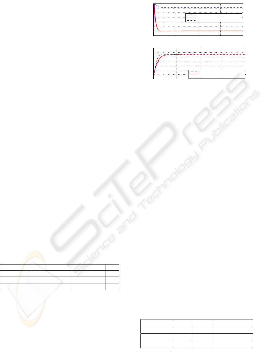
One series of simulations is described (Fig. 2) the
initial condition are the following:
Q
e
(0) = 2m
3
.s
−1
, Q
e
(L) = 0.7m
3
.s
−1
, H
e
(0) =
1.41m, z
e
(L) = 1.8m.
The steady state to reach is defined by:
¯
Q(0) = 2m
3
.s
−1
,
¯
Q(L) = 0.7m
3
.s
−1
,
¯
H(0) = 1.85m,
¯
H(L) = 2.26m.
Using (31), we note that the tuning parameters should
satisfy k
0
k
L
< k
0
k
L
max
= 0.1682.
0 0.5 1 1.5 2
x 10
5
1.8
2
2.2
2.4
2.6
2.8
3
3.2
time (s)
(m
3
.s
−1
)
Upstream Water Flow
reference
With Integral Action
Without Integral Action
0 0.5 1 1.5 2
x 10
5
1.7
1.8
1.9
2
2.1
2.2
2.3
2.4
(m)
Downstream water level
reference
With Intergal Action
Without Integral Action
Figure 2: Water flow at upstream and level at downstream.
Two simulations are pictured, with the following
values k
0
k
L
= 0.0039, and
1. m
0
= 0 = m
L
,
2. m
0
= −0.0001 m
L
= 0.001.
Other simulations with higher values of k
0
k
L
(k
0
k
L
>
k
0
k
L
max
) diverge in the sense that the water flow and
level do not converge to the steady state required or
oscillate.
All the simulations shows the well suitability of the
two stability tests (27)-(28) and of the condition(31),
the three have to be verified to insure the stability of
the system.
The stability hypothesis (16)-(18) linked to the inte-
gral actions are checked, even if it is applied to the
non linear system.
5.2 Experimental Results on a
Micro-channel
An experimental validation has been performed on
the Valence micro-channel (Tab.2). This pilot chan-
nel is located in Valence (France). It is operated
under the responsibility of the LCIS
1
laboratory.
This experimental channel (total length=8 meters) has
an adjustable slope and a rectangular cross-section
(width=0.1 meter). The channel is ended at down-
stream by a variable overflow spillway and furnished
with three underflow control gates (Fig. (3) ).
Table 2: Parameters of the channel of Valence.
parameters B(m) L (m) K (m
1/3
.s
−1
)
values 0.1 7 97
parameters µ
U
0
µ
U
L
slope (m.m
−1
)
values 0.6 0.73 1.6
0
/
00
1
Laboratoire de Conception et d’Int
´
egration des
Syst
`
emes
ICINCO 2007 - International Conference on Informatics in Control, Automation and Robotics
324
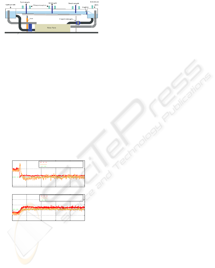
Figure 3: Pilot channel of Valence.
One experimentation has been chosen to illustrate
this approach.
Note that water flow is deduced from the gate
equations, and has not been measured directly. The
data pictured below have been filtered to get a better
idea of the experimentation results.
In each experiment, the system is initially in open
loop at a steady state:
Q
e
(0) = 2.5dm
3
.s
−1
, H
e
(0) = 1.1dm, H
e
(L) = 1.26dm.
The loop is closed at time t = 50sec with a new set
point given by:
¯
Q(0) = 2dm
3
.s
−1
,
¯
H(0) = 1.3dm,
¯
H(L) = 1.43dm.
Two experimentations are pictured in Fig. (4), with
maxk
0
k
L
= 0.888 and the following values:
1. k
0
k
L
= 0.247 & m
0
= 0, m
L
= 0,
2. k
0
k
L
= 0.247 & m
0
= −0.002, m
L
= 0.001.
0 100 200 300 400 500
1.5
2
2.5
3
Water flow at upstream
Time (s)
(dm
3
.s
−1
)
without Integral Action
with Integral action
reference
0 100 200 300 400 500
1
1.2
1.4
1.6
1.8
2
Downstream water
Time (s)
(dm)
without integral action
with integral action
reference
Figure 4: Water flow at upstream and level at downstream.
To conclude this part, let notice that for the micro-
channel, both tests (27)-(28) are quiet equivalent (is
not the case for rivers like the Sambre in Belgium). In
all the cases, one conclusion is the same, the stability
of the system is insured if both tests (27)-(28) and the
condition (31) are realized.
Exact convergence is ensured if the integral part of the
control is added even if it is applied to the real and so
the non linear system.
6 CONCLUSION
In this paper, a boundary control law with integral ac-
tion is proposed, as a new stability condition depend-
ing on the Riemann coordinates. Simulations and ex-
perimentations realized strengthen on the fact that the
stability conditions (16)-(18) can be developed to fit
to the non linear case. Improvements will be the de-
velopment of the works on (Dos Santos et al., 2007)
to non linear system of conservation laws, and/or to
couple both previous results and generalize them to
greater dimension systems.
ACKNOWLEDGEMENTS
The authors would like to thank professor E. Mendes
and the LCIS to have allowed us to realize our exper-
imentations on the micro-channel. In the same way,
thanks to the Cemagref for the use of the software
SIC.
REFERENCES
Coron, J. M., d’Andr
´
ea Novel, B., and Bastin, G. (2007).
A strict Lyapunov function for boundary control of
hyperbolic systems of conservation laws. Automatic
Control, IEEE Transactions on Automatic Control,
52(1):2–11.
Coron, J.-M., de Halleux, J., Bastin, G., and d’Andr
´
ea
Novel, B. (2002). On boundary control design for
quasi-linear hyperbolic systems with entropies as Lya-
punov functions. Proceedings 41-th IEEE Confer-
ence on Decision and Control, Las Vegas, USA,, pages
3010 – 3014.
Dos Santos, V., Bastin, G., Coron, J.-M., and d’Andr
´
ea
Novel, B. (2007). Boundary control with integral ac-
tion for hyperbolic systems of conservation laws: Lya-
punov stability analysis and experimental validation.
submitted to Automatica.
Dos Santos, V. and Prieur, C. (2007). Boundary control of
a channel: practical and numerical studies. in prepa-
ration.
Litrico, X., Fromion, V., Baume, J.-P., Arranja, C., and Rijo,
M. (2005). Experimental validation of a methodol-
ogy to control irrigation canals based on saint-venant
equations. Control Engineering Practice, 13:1425–
1437.
Prieur, C., Winkin, J., and Bastin, G. (2006). Boundary
control of non-homogeneous systems of conservation
laws. preprint.
Renardy, M. and Rogers, R. (1993). An introduction to par-
tial differential equations. Springer Verlag.
BOUNDARY CONTROL OF A CHANNEL - Last Improvements
325
