
DYNAMIC REAL-TIME REDUCTION OF MAPPED FEATURES IN A
3D POINT CLOUD
Marko Reimer and Bernardo Wagner
Institute for Systems Engineering, Leibniz University Hanover, Hanover, Germany
Keywords:
3D perception, real-time processing, data reduction.
Abstract:
This paper presents a method to reduce the data collected by a 3D laser range sensor. The complete point
cloud consisting of several thousand points is hard to process on-line and in real-time on a robot. Similar
to navigation tasks, the reduction of these points to a meaningful set is needed for further processes of object
recognition. This method combines the data from a 3D laser sensor with an existing 2D map in order to reduce
mapped feature points from the raw data. The main problem is the computational complexity of considering
the different noise sources. The functionality of our approach is demonstrated by experiments for on-line
reduction of the 3D data in indoor and outdoor environments.
1 INTRODUCTION
Environmental perception of mobile robots is still a
challenging task. Many research groups work on im-
provements for on-line spatial perception. Almost all
possible kinds of sensors are used to collect informa-
tion. Actually, lots of research in robotics deals with
the localization and mapping problem. Partly, this re-
search is based on features. These features are mostly
lines, planes or special edges. Few research is done in
processing all the raw data in real-time on the robot
itself. The main problem for doing it on-line is the
less time for each process combined with less com-
putation power for each step to finish. A further field
of research, mainly in security context, focuses on ob-
ject detection. On-line algorithms for object detection
must be integrated into the control process to be of
any advantage for robot task fulfillment and have to be
finished in real-time time. One of the most important
steps to speed up the data processing is to reduce the
collected data to a meaningful set of data. An exam-
ple for this is the mapping and localization problem.
Therefore feature points in 3D are extracted, mapped
into a 2D map and well known 2D algorithms are ap-
plied (Wulf et al., 2004b). The intention of this paper
is to present a way to reduce the amount of data col-
lected by a 3D range scanner for a following on-line
object detection. This reduction uses environmental
context knowledge to remove static features like walls
from the 3D point cloud and keep only information
not present in the given map. This may be used for re-
ducing speed of an autonomous vehicle within range
of dynamic obstacles. The reduceable feature points
are found by two criteria. First, several sequent points
must form a vertical line in 3D space. Second, this
line must be matched to the environment map of the
robot. As the computation power and the data stor-
age for on-line reduction is limited, only actual data
is used without keeping any previous information or
calculating averages over time.
Another benefit reducing the raw data, additional
to the gain in speed, is the better result of algorithms
working on the reduced data set. A following ob-
ject detection and segmentation algorithm may not be
confused by mapped (known) features any more. For
an example segmentation see (Talukder et al., 2002).
The main problem handled in this paper is match-
ing the 3D-data in the presence of different kinds of
noise. All used sensors and maps have different forms
of noise requiring different handling.
The paper is organized in 5 parts. The remaining
part of section 1 describes the form of the input data.
Section 2 describes similar work. Section 3 shows
the steps needed for the reduction and ways to handle
363
Reimer M. and Wagner B. (2007).
DYNAMIC REAL-TIME REDUCTION OF MAPPED FEATURES IN A 3D POINT CLOUD.
In Proceedings of the Fourth International Conference on Informatics in Control, Automation and Robotics, pages 363-369
DOI: 10.5220/0001638003630369
Copyright
c
SciTePress

uncertainties. After that, the experiments carried out
on two robot platforms one indoor and one outdoor
are shown in section 4. The conclusion is drawn in
the 5. section.
The 3D data to be reduced is measured from a
continuous 360 degree 3D laser range scanner. To be
able to collect data while moving a movement com-
pensation is applied. For details on the 3D sensor and
the movement compensation see (Wulf and Wagner,
2003) or (Reimer et al., 2005). A 3D scan is organized
as an ordered sequence of vertical 2D laser scans (see
Figure 1 left) in clockwise rotating directions. One set
of 3D data always contains a 360 degree turn of the
3D scanner. Each 2D laser scan itself is an ordered
list of points in 3D space. There is a fixed number of
points per 2D scan which are ordered from bottom di-
rection towards ceiling direction. The points are given
in cartesian coordinates with the origin centered at the
laser scanner.
Like a normal 2D map the map used for reduction
represents the environment in a top view. The map
consists of a set of lines defining surfaces detectable
by a range sensor (see Figure 1). As the map is de-
signed and also used for localization it only needs to
include a 2D representation of the environment. This
kind of map is often build from landmark offices or
construction plans, which are not including 3D infor-
mation. It might be build from aerial images given
ground truth.
Figure 1: Left: Schematic of a 2D/3D Scan; Right: Sample
map of our office environment.
2 RELATED WORK
At the first step, each 2D scan is handled seperately.
Each 2D scan is segmented into lines. These line
features extracted from range data are used by sev-
eral successful systems as they are easy to compute
and quite compact to handle. There are several pa-
pers how to construct line features. Two of the most
commonly used ways are either Hough transforma-
tion (Pfister, 2003), and the split-and-merge approach
(Borges, 2000). For an overview of line segmentation
algorithms see (Nguyen et al., 2005).
The closest work to ours is the work extracting
walls from 3D points collected by a static mounted
but moved 2D scanner. For example (Thrun, 2003)
collect these data with a helicopter, and Haehnel et al.
do so with a moving robot (Haehnel et al., 2003). The
main difference is the way 3D points are built. In their
case the whole system is moved along a given path
while the sensor is static on the system. They achieve
a more dense point cloud and have a reduced angular
error. They do not reduce the data on-line and in real-
time but they post process the whole point cloud to
extract matched walls using the EM-algorithm.
The proposed method should remove as much
points as possible of visible matching feature parts.
In contrast to the shown wall matching methods with
a minimum 2D size, our method needs only a line to
be detectable. The overall height of a line or plane is
not constrainted. The removed features are not con-
stricted by any minimum size requirement as it de-
pends on the distance to the feature.
Another similar technique is the well researched
segmentation of horizontal 2D range data into line
features and matching them with a given 2D map.
This is mostly done for localization like (Biber, 2005)
and (Pfister, 2003). This is at least done on-line
while the system operates. In the case of a vertical
mounted 2D scanner vertical and not horizontal lines
are measured, which differ in handling. Horizontal
line matching has to deal with similar sensor noise
and errors in the position estimation. But the horizon-
tal neighborship of succeeding points can be used to
account for the angular error in the localization. Com-
pared to a horizontal neighbouring point a whole line
in the vertical scan is effected by this error. The line
cannot be corrected by weighting the single point with
neighboring points into a line.
On the first sight, the well researched area of map-
ping is very similar to the described problem. There
is an enormous number of papers about ‘SLAM’
which are at least partly dealing with the problem of
mapping ((Thrun et al., 2005), (Thrun et al., 2004),
(Nuechter et al., 2005), (Kuipers and Byun, 1990)).
Especially the survey (Thrun, 2002) gives a good
overview. The main difference of our approach to
the mapping problem is that we assume to know our
position and orientation up to a remaining error in-
troduced by the localization. It is not our attempt to
improve the quality of the localization in any kind
as we want to detect and segment dynamic objects.
The SLAM takes a big advantage of the possibility
to sense a particular point in space twice or more of-
ten. As shown in (Thrun, 2002) they take an EM-
algorithm to maximize the probability of a particular
cell in a grid map. This is manly done using multiple
ICINCO 2007 - International Conference on Informatics in Control, Automation and Robotics
364
views of the same cell over time. We want to reduce
data immediately. These SLAM algorithms include
methods for an estimated match of 2D point positions,
mostly positions of feature points, with a given 2D
map of the environment for localization (Wulf et al.,
2004a).
Another similar topic is the iterative matching of
two 3D scans or the iterative matching of features to
3D scans. There exist lots of matching techniques.
The most popular technique is the iterative closest
point (ICP) algorithm based on (Besl and McKay.,
1992). As all these techniques try to give an optimal
result in the overall match it takes too much computa-
tion time for our application.
3 REAL-TIME REDUCTION OF
3D DATA
Assuming a perfect localization, a perfect map and a
noiseless sensor, the mathematical model for the re-
duction of 3D data to a 2D-map is straightforward. If
the sensor is located at position α and the measured
points form an exact vertical line at position β both
positions can be transformed into positions within the
map without any error. The position of the robot in
the map is ι and the feature position is called δ. It is
a comparison between the measured distance and the
distance given by the map assuming the same direc-
tion.
d
αβ
− d
ιδ
= ζ (1)
If ζ is smaller than a threshold, the points are re-
moved.
3.1 Laser Scanner Noise
The most common problem is the measurement noise
of the laser range sensor. We show here how to care
about the sensor noise without explizitly handling ev-
ery point but combining the errors into a line repre-
sentation. Range sensors mostly report data in a po-
lar representation consisting of a distance measure-
ment and a corresponding measurement angle. The
distance measurement of commonly used laser scan-
ners underlies a gaussian noise as shown in (Ye and
Borenstein, 2002). This noise depends on parame-
ter as temperature, incidence angle and color of the
scanned surface. They showed that the influence of
the surface properties is less than the influence of the
incidence angle. As for example in (Pfister, 2002) the
noise of a 2D laser scanner in the measured angle can
be modeled as an additive zero-mean gaussian noise
with a variance of σ
2
. Whereas a common assumption
σ
2
is less than one degree. The resulting measured
distance vector
d
meas
is calculated by
d
meas
= (d
true
+ ε
d
sensor
) ×
cos(Θ+ ε
Θ
)
sin(Θ+ ε
Θ
)
(2)
with Θ being the assumed angle of the measure-
ment and ε being the corresponding error. For our
reduction we do not consider single points and their
noise but lines. These lines allow us to handle the
sensor noise as an distance interval in the 2D ground
distance d
ground
meas
.
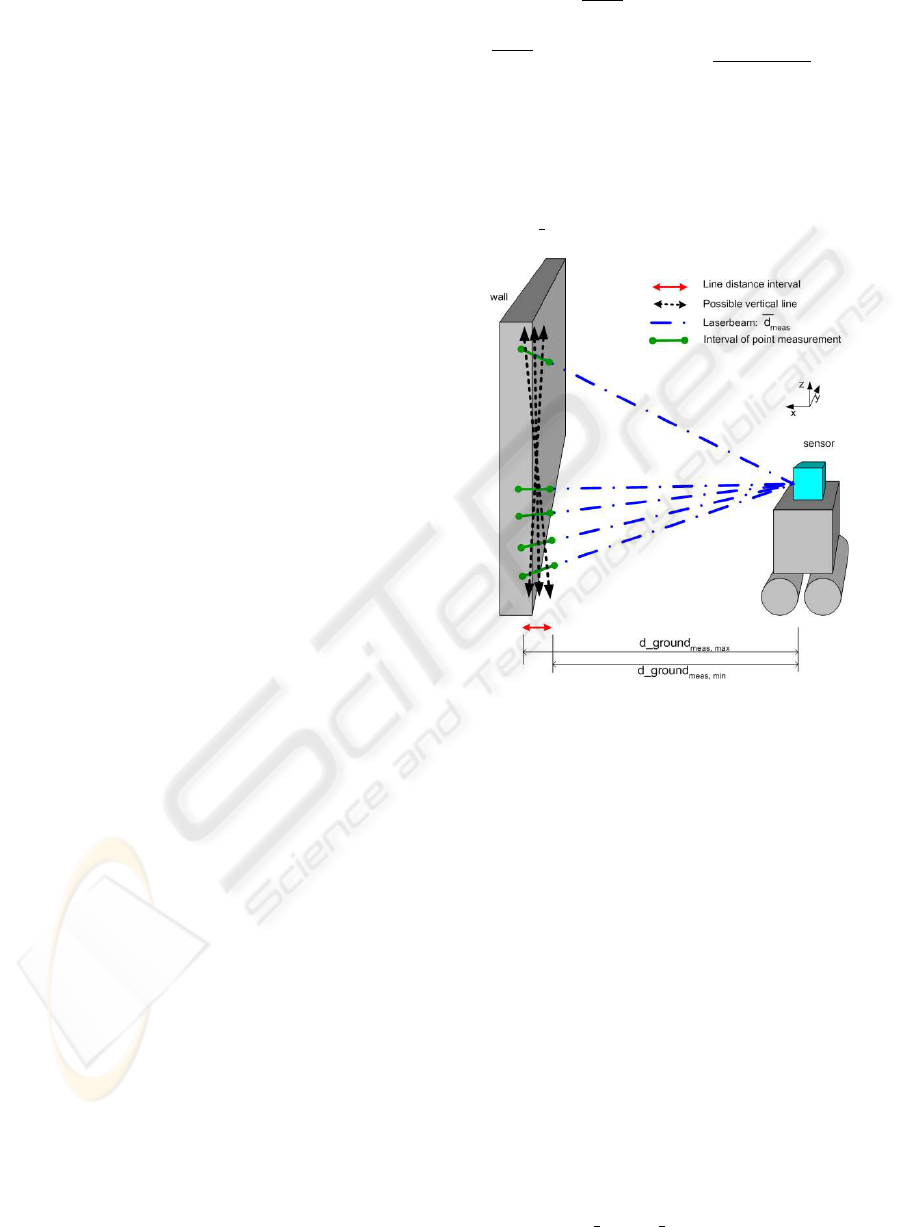
Figure 2: Sensor noise - points forming lines.
Figure 2 shows an example of the possible distri-
butions of some wall points. As all points are taken
on the front side of the wall they must be measured
at the real distance added gaussian noise. The pos-
sible locations of the scanned points are shown by
the intervals around the true front point at the wall
(green solid lines). The line search algorithm is con-
figured to some maximum distance a measured point
may have towards the line. This defines the spread
of points around the line. After fitting a line through
the points the upper and the lower end point of the
line define the maximum and minimum distance of
the line to the sensor. There are several orientation
possibilities for the found line, depending on the dis-
tribution of the noise (dotted orange lines). The angle
of the found line against the z-axis is named γ. It’s
bound by a userdefined treshold η. This line forms
the measured ground distance interval at the xy-plane
(red line). This interval is given by:
d
ground line
meas, j
= (3)
DYNAMIC REAL-TIME REDUCTION OF MAPPED FEATURES IN A 3D POINT CLOUD
365
[min
i
(d ground
meas,i
);max
i
(d ground
meas,i
)]
with i all points forming line j.
The mounting of the scanner does not need to be
exactly vertical. So an error in the orientation of the
lines is introduced. This angular difference is directly
visible in the orientation of the measured line (orange
line in Figure 2. All lines are not exactly vertical any-
more but tilted. The tilting angle adds to the interval
of possible line orientation angles (γ). This angular
error results in different distances for the upper and
lower ending of the line. The error in the distance is
dependent on the length or height of the wall and the
height of the scanner position. This error has a maxi-
mum influence, if both ends of the line strongly differ
in the height towards the sensor. As an example a 2
degree mounting error results in a 10 cm distance er-
ror, if the line has a height of 3 m, if the scanner is
mounted on the ground. This distance difference adds
to the distance interval caused by the sensor distance
noise.
d
error
(γ) = height ∗ tan(γ) (4)
As the tilting of the sensor is detectable during the
mounting process it can be mechanically bound. To
simplifiy calculations this maximum bound is used.
The minimum distance is given by:
d
total
meas,min
= d ground line
meas,min
− d
error
(γ)
(5)
Similar calculations can be applied for the maximum
distance. Together these two values form the mea-
sured distance interval.
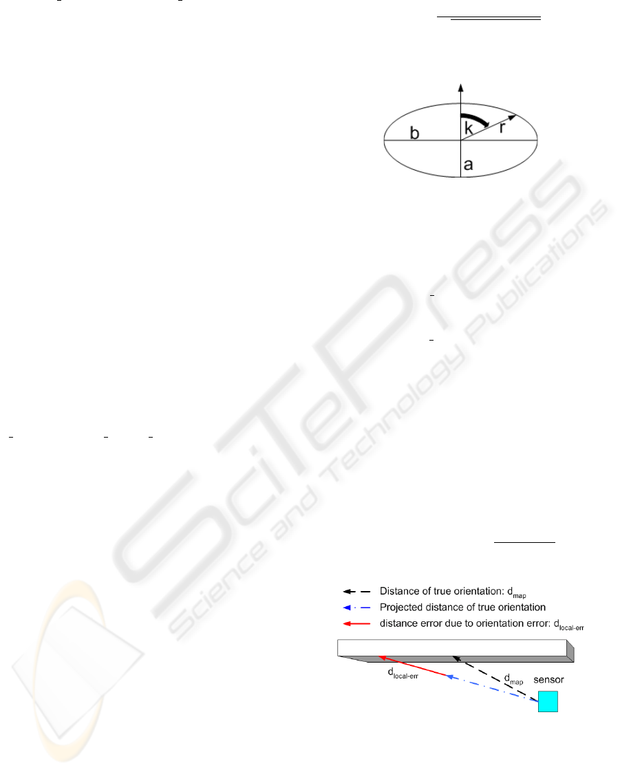
3.2 Localization Distance Noise
For calculating the expected distance the map and the
output of the localization are used. These values are
independent of the sensor model. As our algorithm
relies on a given localization, we must take the error
of the localization into account. A commonly used
model for the localization error (Thrun et al., 2005)
describes the located position as an ellipse with axis
a and b, the orientation as an angle ω added a zero-
mean gaussian noise ε
ω
. There is no general bound on
the localization error which can be applied to all dif-
ferent kinds of localization methods. So we assume
these variances to be known for each position. As
we want to reduce data very fast, we do not try to
upgrade the position data by any means. We use the
radii of the ellipses to calculate the possible difference
in the ground distance introduced by the localization
and build an interval of this size around the reference
value taken from the map using the center of the el-
lipse.
r
position
=
b
p
1− a
2
b
2
cos
2
(κ)
(6)
κ is the direction of the scan. It is counted clockwise
from the front direction of the scanner.
Figure 3: Localization position error.
The condition for the reduction is given by equa-
tion 7, when the angular error of the localization is
not considered.
(d
map
− r
position
≤ d total
meas,min
≤ d
map
+ r
position
)
or (7)
(d
map
− r
position
≤ d
total
meas,max
≤ d
map
+ r
position
)
3.3 Localization Orientation Noise
The angular difference between the true orientation
and the measured orientation has a worse effect than
the position error. On a plane object or wall this angu-
lar error introduces a difference in the incidence angle
ρ between the beam and the object. The resulting er-
ror in the distance is dependent on the distance and
the actual incident angle.
d
local−err
= d
map
×
1−
sin(ρ)
sin(ρ+ ε
ρ
)
(8)
Figure 4: Incidenceangle with orientation error.
This error might be of enormous impact for small
incident angles at large distances. If we add the dif-
ference d
local−err
(8) to the already calculated interval
by Section 3.2 it is no longer possible to distinguish
between objects significant in front of the wall and
the wall itself. If we do not consider this error, the
ICINCO 2007 - International Conference on Informatics in Control, Automation and Robotics
366
points forming this line are not reduced and remain
for further processing steps. To account for this we
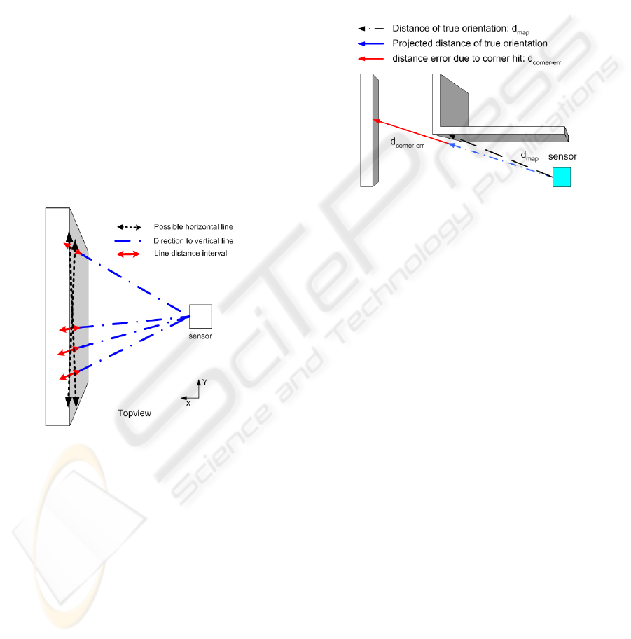
extend the identified lines from the measured points.
Our approach is to form a horizontal line from the al-
ready found vertical lines. The found vertical lines
are projected into the ground plane. They form an
interval or line in the xy-plane in contrast to the line
in the xyz-system in Figure 2. All already matched
wall lines are marked like the blue lines in Figure
5. The centers of neighboring matched ground lines
are tested for forming a horizontal line in the ground
plane using the same methode as in the first part. The
next vertical line not already matched is tested to be a
part of this horizontal line. Doing this the difference
between the unmatched vertical line distance and the
horizontal line is bounded by the point distance dif-
ference and independent of the distance error between
the map and the measurement. If the vertical line in-
terval fits into the horizontal line it is reduced as well.
This method needs the feature to be matchable at least
party. A matched segment must form a line to be ex-
tended.
Figure 5: Vertical lines forming horizontal line.
3.4 Remaining Noise Sources
The error in the estimation of the measurement angle
introduced by the servo drive cannot be handled in the
same way as the orientation error of the localization.
This error depends on the sampling frequency of the
servo drive position and it is acceleration. The posi-
tion of the servo drive is linear interpolated between
two measurements. If the servo drive accelerates the
change in turn velocity leads to an angular error de-
pendent on the acceleration speed and sampling fre-
quency of the position sensor. Both variables are con-
trollable by the user and may be chosen to result in
a negligible angular error. This might be reached, if
the system is considered to be turning with a constant
turn velocity after a startup phase.
The worst problem appears, if the angular differ-
ence between map and measured beam results in a hit
on a different object or wall due to a corner. In this
case the mathematical expression of the differences
in the distance are not longer valid. Partly, if the inci-
dence angle is small enough this case is caught by the
horizontal line extension. The lines not caught remain
as line in the point cloud.
Figure 6: Error hitting a corner.
The mixed pixel problem is not solved by our ap-
proach. A measured line of points within a mixed
pixel distance to the sensor cannot be matched to any
feature. As the remaining vertical lines are orphants
within their neighbourhood, they might be removed
in a postprocessing step.
Finally, the map itself is probably not perfect but
has some error. The error within the map is assumed
to be within the same dimension as the noise of the
range sensor. And therefore not handled explizit.
4 EXPERIMENTS
The proposed method has been implemented into the
perception module of our 3D laser scanner. This 3D
laser scanner is mounted on to two different chassis
one for indoor use Section 4.1 and one for outdoor use
Section 4.2. Both systems differ in various parameter
but use the same software environment. For the in-
door cases the map is created by hand using manually
measured length. The outdoor map is based on mate-
rial from the land registry office. The map error is in
the dimension of centimeter. The same maps are used
for localization and reduction at all times. The 3D
laser scanner consists of a Pentium III Processor with
256 MB of RAM running a real-time linux (Xeno-
mai). The time needed for the reduction on this pro-
cessor is well below one second.
DYNAMIC REAL-TIME REDUCTION OF MAPPED FEATURES IN A 3D POINT CLOUD
367
4.1 Indoor Experiments
For the indoor experiment we were driving on the
floor with a speed of 0.5 m/s when the 3D scan has
been taken. Beside the walls and doors there is one
person and one cartoon standing on the floor roughly
in front of the robot. The doors on the left side are
closed, while the doors on the right are open. Through
the right door an office is visible. This office is
equiped with normal filled desks and cabinets at the
wall. On the back side a fire extinguisher is located at
the wall.
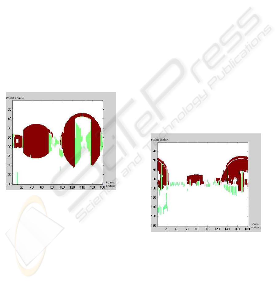
Figure 7 shows all found vertical lines and the re-
sult of the reduction. The dark red lines have been
matched to the map while light green lines remain
unmatched. At a first glance some lines within the
wall appear not vertical. This is a problem of the line
segmentation algorithm. As shown in (Borges, 2000)
the start and endpoints of a line are not always chosen
correctly. This may result in a wrong angle calculated
for that line. These single lines (the corresponding
points) will be removed after the matching step.
Figure 7: Reduced(red) and remaining lines(green) indoor.
On the left hand side all but one small vertical line
on the wall has been removed. The door in the front
part has not been modeled in the map and cannot be
reduced at all. (see Figure 1) Also the person and
the carton still remain as detected lines. The open
door on the right remains like the lines on the cabinets
within the office. The wall on the right side is totally
removed even far in front at small incidence angles.
This is due to the applied wall extension. The far wall
on the left side cannot be removed because the person
is totaly blocking the wall extension. On the back side
on the left, between Scanindex 0-1, some lines which
belong to a wall have not been removed. This is due to
the error in the orientation while processing a corner
in the map. At this direction no wall is found. The
calculated beam hits the right side of the corner with
the front wall, while the measured beam passes on the
left side to the about 5m far away wall. The small
line not removed around scanIndex 22 belongs to an
other open door. In total from 12300 points forming
vertical lines about 11700 points are removed. The
complete 3D scan has 32761 points.
4.2 Outdoor Experiments
For the outdoor experiments we drove around a park-
ing lot with several warehouses around. These build-
ings form the vertical lines to be matched. All existing
features have been found as lines. As the distance to
the buildings is big compared to the indoor distances
much less points form vertical lines. All found ver-
tical lines are shown in Figure 8. The removed ver-
tical lines are dark red and remaining vertical lines
are light green. These remaining lines are mostly lo-
cated at the wirefence on the right side and the bush
on the front side. Both are not represented in the map
to be removed. The white area shows points not iden-
tified as vertical line and so not applictable for our
reduction. All existing features have been removed
while all dynamic objects are remaining. The com-
putational complexity of further steps is reduced by
more than 50 percent as most of the significant points
are removed.
Figure 8: Reduced (dark red) and remaining lines (light
green) outdoor.
5 CONCLUSION
In this paper we presented a method for real-time and
on-line reduction of a 3D point cloud by given rough
2D-environmental knowledge. The method finds ver-
tical line features in the 3D data and matches them
to a given 2D map of these features. The problem
ICINCO 2007 - International Conference on Informatics in Control, Automation and Robotics
368

for this procedure is the different noise introduced by
several measurements. In order to speed up the calcu-
lation and simplifiy to noise handling we do not deal
with every single point but build higher level line fea-
tures. These line features are suitable to incorporate
the noise added to the distance measurements. The
line approach is used a second time on the line fea-
tures itself, in order to handle the error in the orien-
tation angle. The vertical lines are reduced to points
on the ground which form a horizontal line feature to
be independent of the relative orientation. A possible
extension could be the integration of a non straight
feature model as for example curved walls.
The proposed method is well suited for dynamic
and complex environments as long as a simple 2D-
map of matchable features is given and these features
remain visible beside the dynamic objects. It im-
proves a following object detection and recognition
in computational speed and result quality.
The best improvement for the reduction quality
may be gained by an improvement of the localization.
Until the localization error is in the same dimension
as the sensor noise, the use of a second or better sen-
sor is not usefull. A possible extension might be to
use the intensity value delivered by a range sensor to-
gether with the distance value. This intensity value
is proportional to the strength of the reflection of the
transmitted signal. The uncertainty interval of a mea-
sured distance could be calculated corresponding to
the measured intensity of the distance. But the in-
tensity is dependent on many factors not only on the
incident angle and the other influences have to be can-
celed out before.
REFERENCES
Besl, P. J. and McKay., N. D. (1992). A method for
registration of 3-d shapes. IEEE Trans. on PAMI,
14(2):239256.
Biber, P. (2005). 3d modeling of indoor environments for
a robotic security guard. Proceedings of the 2005
IEEE Computer Society Conference on Computer Vi-
sion and Pattern Recognition (CVPR05).
Borges, G.A; Aldon, M.-J. (2000). A split-and-merge seg-
mentation algorithm for line extraction in 2d range im-
ages. Pattern Recognition, 2000. Proceedings. 15th
International Conference on, pages 441–444.
Haehnel, D., Triebel, R., Burgard, W., and Thrun, S. (2003).
Map building with mobile robots in dynamic environ-
ments. ICRA.
Kuipers, B. and Byun, Y.-T. (1990). A robot exploration
and mapping strategy based on a semantic hierarchy
of spatial representations. Technical Report AI90-120.
Nguyen, V., Martinelli, A., Tomatis, N., and Siegwart, R.
(2005). A comparison of line extraction algorithms
using 2d laser rangefinder for indoor mobile robotics.
International Conference on Intelligent Robots and
Systems, IROS2005,.
Nuechter, A., Lingemann, K., Hertzberg, J., and Surmann,
H. (2005). 6D SLAM with approximate data associa-
tion. ICRA.
Pfister (2002). Weighted range sensor matching algorithms
for mobile robot displacement estimation. Interna-
tional Conference on robotics and automation, pages
1667–1675.
Pfister, Samuel; S. Rourmelitis, J. B. (2003). Weighted line
fitting algorithms for mobile robot map building and
efficient data representation. International conference
on robotics and automation, pages 1304–1312.
Reimer, M., Wulf, O., and Wagner, B. (2005). Continuos
360 degree real-time 3d laser scanner. 1. Range Imag-
ing Day.
Talukder, A., Manduchi, R., Rankin, A., , and Matthies,
L. (2002). Fast and relaiable obstacle detection and
segmentation for cross-country navigation. Intelligent
Vehicle Symposium, Versaille, France.
Thrun, S. (2002). robotic mapping a survey. Book chap-
ter from ”Exploring Artificial Intelligence in the New
Millenium”.
Thrun, S. (2003). Scan alignment and 3-d surface modeling
with a helicopter platform. IC on Field and service
robotics, 4th.
Thrun, S., Burgard, W., and Fox, D. (2005). Probabilistic
Robotics. The MIT Press.
Thrun, S., Montemerlo, M., Koller, D., Wegbreit, B., Ni-
eto, J., and Nebot, E. (2004). Fastslam: An efficient
solution to the simultaneous localization and mapping
problem with unknown data association. Journal of
Machine Learning Research.
Wulf, O., Arras, K. O., Christensen, H. I., and Wagner, B.
(2004a). 2d mapping of cluttered indoor environments
by means of 3d perception. ICRA.
Wulf, O., Brenneke, C., and Wagner, B. (2004b). Col-
ored 2d maps for robot navigation with 3d sensor data.
IROS.
Wulf, O. and Wagner, B. (2003). Fast 3d scanning methods
for laser measurement systems. International Con-
ference on Control Systems and Computer Science
(CSCS), 1.
Ye, C. and Borenstein, J. (2002). Characterization of a
2-d laser scanner for mobile robot obstacle negotia-
tion. International Conference on Robotics and Au-
tomation.
DYNAMIC REAL-TIME REDUCTION OF MAPPED FEATURES IN A 3D POINT CLOUD
369
