
MINIMIZING THE ARM MOVEMENTS OF A MULTI-HEAD
GANTRY MACHINE
Timo Knuutila, Sami Py
¨
otti
¨
al
¨
a and Olli S. Nevalainen
Department of Information Technology, University of Turku, FI-20014 Turku, Finland
Keywords:
Printed circuit board, electronics assembly, multi-head placement machine, optimization, production control.
Abstract:
In printed circuit board (PCB) manufacturing multi-head gantry machines are becoming increasingly more
popular in surface mount technology (SMT), because they combine high speed with moderate price.
This kind of machine picks up several components from the feeder and places them on the PCB. The process
is repeated until all component placements are done. In this article, a subproblem of the machine control is
studied. Here, the placement order of the components, the nozzles in the placement arm and the component
locations in the feeder are fixed. The goal is to find an optimal pick-up sequence when minimizing the total
length of the arm movements.
An algorithm that searches the optimal pick-up sequence is proposed and tested widely. Tests show that the
method can be applied to problems of practical size.
1 INTRODUCTION
The electronics industry has been one of the fastest
growing fields of industry in the last 20 years. Here,
one of the central fields is the manufacturing of
printed circuit boards (PCBs) which are needed ev-
erywhere in present days. Electronic components are
installed to PCBs with specialized, automated com-
ponent placement machines. Production batches of
similar PCBs can be very large especially in the mass
production of consumer electronics. PCBs can be
manufactured with a single machine or more com-
monly with an assembly line of several consecutive
machines of different types. An assembly line con-
sists of a solder paste printer, a few placement ma-
chines and an oven in which the components are fixed
onto the board. Usually, each placement machine is
specialized to place a certain set of component types.
In the past, components were attached to PCBs
mainly using through-hole technology (THT) but
nowadays, when minituarizing the products, the in-
dustry has changed over to surface mount technol-
ogy (SMT). In order to be successful, the component
placement operations require great accuracy from the
placement machine, because components and PCBs
have become smaller and smaller. While technology
has developed, different types of placement machines
have been invented, including dual-delivery, multi-
station, turret-type, and multi-head gantry machines.
Each machine type has its own special features and is
suitable for different types of assembly tasks, see e.g.
(Ayob et al., 2002) and (Ayob and Kendall, 2005) for
discussion.
The operation of a placement machine is con-
trolled with a control program which states the de-
tails of individual component placement steps. This
program should force the machine perform its task as
fast as possible while still satisfying high quality stan-
dards. A single PCB can include dozens of different
kinds of components and the total number of compo-
nents on one PCB can amount to several hundreds.
The actual placement of a component requires the use
of a suitable nozzle. One or more nozzles are at-
tached to the placement head of a machine. Normally,
nozzles can be changed when necessary. In some
machines the nozzle changes have to be done man-
ually while some others can change them automat-
ically. The placement machine fetches components
from a feeder unit capable of holding a large number
of copies of components of each type and then places
326
Knuutila T., Pyöttiälä S. and S. Nevalainen O. (2007).
MINIMIZING THE ARM MOVEMENTS OF A MULTI-HEAD GANTRY MACHINE.
In Proceedings of the Fourth International Conference on Informatics in Control, Automation and Robotics, pages 326-335
DOI: 10.5220/0001638903260335
Copyright
c
SciTePress
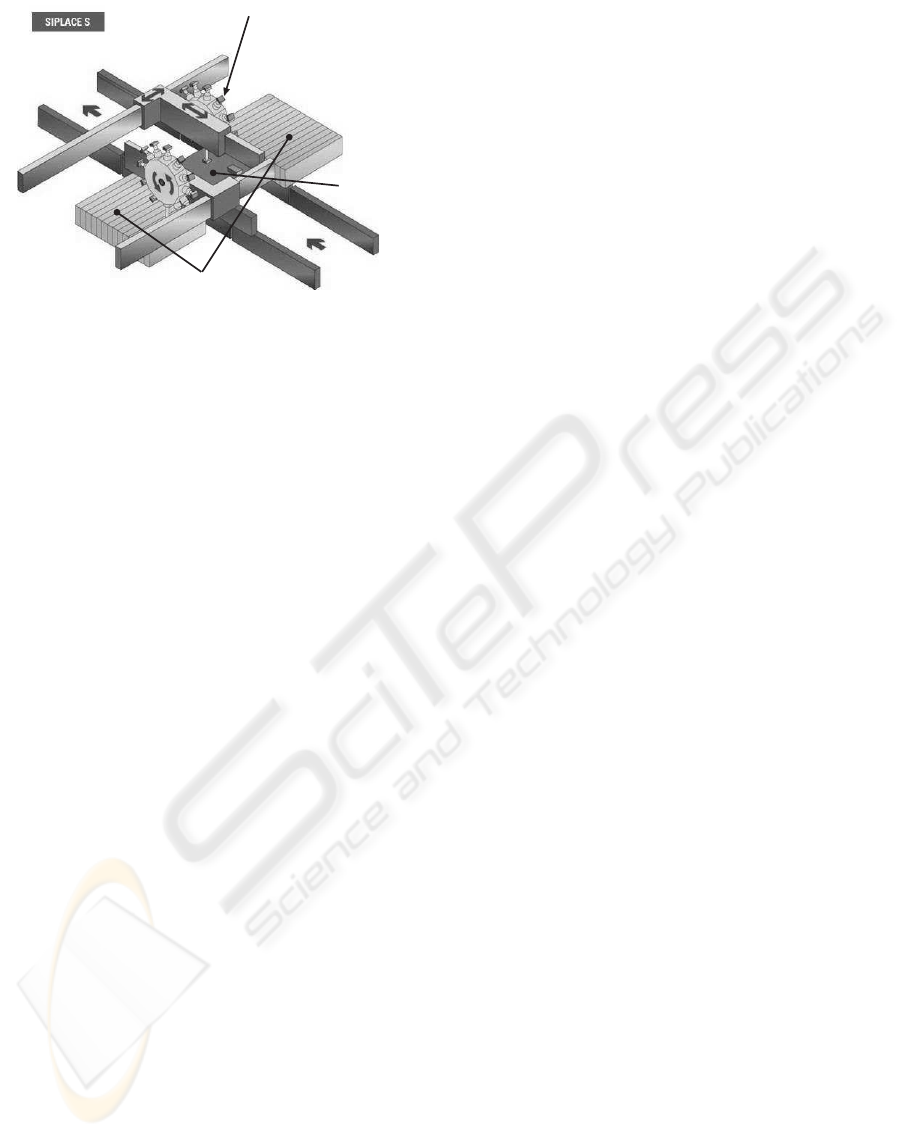
feeders
placementhead
andnozzles
PCB
Figure 1: There are many multi-head gantry machines
in Siplace-series of Siemens. (The image is taken from
Siemens www-page.).
them onto the PCB being manufactured. The determi-
nation of the route the placement head travels during
a placement job can be considered a special asymmet-
ric travelling salesman problem (ATSP) . Solving the
problem requires efficient heuristics that have been
studied in (Ball and Magazine, 1988) (Leip
¨
al
¨
a and
Nevalainen, 1989) for example.
In this article the optimal control of a multi-head
gantry placement machine (Sun et al., 2004) is dis-
cussed. For example Siemens has this type of ma-
chines, see Figure 1 for details. Multi-head gantry
machines have increased their popularity in recent
times due to their flexibility and relatively low acqui-
sition price. In this machine the PCB is positioned
firmly on the stationary table. The machine has a
placement arm with a placement head at one end. The
placement head moves above the PCB and the com-
ponent feeders in (x, y)-plane parallel to the PCB. The
feeders are stationary and arranged as a linear array
along the x-coordinate-side of the PCB fixation table.
There are several (1-30 pieces) spindles (nozzle hold-
ers) in a placement head and each spindle can hold
any type of nozzle. A nozzle can grab a single compo-
nent at a time and different components may require
certain nozzle. Every nozzle of the placement head
can hold a component simultaneously. The placement
head can place one component at a time onto a PCB
and it must then move to the position required by the
next component. While performing a placement job
the machine will retrieve multiple components at a
time from the feeders into the nozzles of the place-
ment head and place them to predetermined positions
on the PCB. This process will be repeated as many
times as necessary. See (Py
¨
otti
¨
al
¨
a et al., 2005) for
more details on the design of the multi-head gantry
machine.
The controlling of a multi-head gantry machine
can be seen as a sequence of multiple decisions.
These include among others the selection of nozzles,
the feeder arrangement, the component pick-up and
placement sequencing. When the decisions are done
consecutively, each of them depends on the previous
ones. For instance the optimal component pick-up se-
quence depends on the beforehand selected nozzles
and the order in which the components are in feeder.
In this hierarchical way it is possible to find a suffi-
ciently efficient solution for manufacturing a certain
PCB but it will not guarantee a globally optimal solu-
tion in a sence of assembly time of a single job. Even
though the hierarchical method is complicated it has
led to some good results (Kumar and Li, 1995; Crama
et al., 1990; Lee et al., 1999) whereas the joint mod-
elling of this machine type leads to a mathematical
model of impractically high complexity.
The approach used in this article is slightly differ-
ent from previous studies. Our aim is not to solve the
whole control problem but instead to consider a par-
ticular subproblem in greater detail. The subproblem
can be chosen because it is a part of the overall manu-
facturing problem. All subproblems have to be solved
in order to solve the entire problem. In this work, it
is especially asked in which order the multi-head arm
should pick up the components to be placed so that
the movements of the arm are minimized for a certain
printed circuit board (PCB). Two cases are discussed
here. In the first case the sequence for performing the
placements, the nozzles in the placement arm and the
order of component reels in the feeder are predeter-
mined and a pick-up sequence of the components and
its cost shall be computed. This is called the single
pick-up event problem (SPE). In the second case the
assumptions are as above, but the computed pick-up
sequence should be the one with a minimal cost (i.e.
time). This is called the minimal pick-up sequence
problem, MPS. Here again, the optimal machine con-
trol depends on both the placement sequence and the
feeder assignment at the same time, see (Leip
¨
al
¨
a and
Nevalainen, 1989) for discussion of the special case
with a single nozzle in the pick-up-placement head.
In this paper, there are multiple nozzles in the place-
ment head and the arm may contain multiple copies of
the same nozzle type as it is presently common due to
the very skewed distribution of different component
types on PCBs.
The rest of the work is organized as follows. The
notation and terminology are presented in section 2,
as well as the actual research problems. Then in sec-
tion 3 the problems are solved and possible algorithms
are proposed. The best proposed algorithm is tested
and the results introduced in section 4. The final sec-
tion consists of the concluding remarks.
MINIMIZING THE ARM MOVEMENTS OF A MULTI-HEAD GANTRY MACHINE
327

2 MINIMAL PICK-UP SEQUENCE
(MPS) PROBLEM
2.1 Notation and Terminology
The sets of component types and nozzle types are
denoted with C = {c
1
, . . . , c
n
} and T = {τ
1
, . . . , τ
m
},
respectively. A job w is a sequence consisting of
triplets (c, x, y), where c ∈ C and the pair x, y ∈ R
give the location of the component on the PCB. Let
τ(c) be a function defining the nozzle type that has
to be used to pick up a certain component of type c.
Note that different component types (say c
i
and c
j
)
may well require the use of a nozzle of the same type
(τ(c
i
) = τ(c
j
)). The multisets of component types
and nozzle types of job w are denoted with C(w) and
T(w), respectively. They are defined as
C(w) = {chii | (c, x, y) ∈ w}
T(w) = {τ(c)h ji | c ∈ C(w)},
where i and j give the number of copies of the par-
ticular c and τ(c), respectively. An arm a of capac-
ity a
max
is a sequence of nozzle types of length a
max
.
Similarly to jobs, let us denote with T(a) the multiset
of nozzle types in a. Given a job w and an arm a, we
say that a can pick up w if and only if T(w) ⊆ T(a),
that is, there is a nozzle of a correct type in a for each
component type of w. The ⊆-operator is here defined
between multisets (i.e. for each τ(c)h ji ∈ T(w) there
is τ(c)h j
′
i ∈ T(a) such that j ≤ j
′
). Note that the or-
der in which the component types appear in w and a
may be different. Consequently, this means that the
placement order may differ from the pick-up order.
Example. Suppose we have a job
w = (c
1
, x
1
, y
1
)(c
2
, x
2
, y
2
)(c
3
, x
3
, y
3
)(c
4
, x
4
, y
4
),
τ(c
1
) = τ(c
2
) = τ
1
, τ(c
3
) = τ(c
4
) = τ
2
, an arm of
capacity 5, 3 nozzles of type τ
1
and 4 of type τ
2
.
Clearly T(w) = {τ
1
h2i, τ
2
h2i}. Arm a
1
= τ
1
τ
1
τ
1
τ
2
τ
2
can pick up w, since T(w) ⊆ T(a
1
) = {τ
1
h3i, τ
2
h2i}.
On the other hand, arm a
2
= τ
1
τ
2
τ
2
τ
2
τ
2
can not pick
up w, since T(w) 6⊆ T(a
2
) = {τ
1
h1i, τ
2
h4i}.
2.2 Cost of a Pick-up Event
Suppose that we can pick up w using a. We next for-
malize a model for the actual execution of this pro-
cess. We assume for the sake of simplicity that there
is only one source for each component type in the
feeder unit. Then each component type c has a unique
location, say s(c), ranging over the different locations
in the feeder unit. Hence, s is an injective function
s: C → {1, . . . , f
max
}, where f
max
is the total number
of slots in the feeder unit.
The pick-up arm moves first to the location s(c)
of some component type c of the current job w. It
then selects the next of the remaining components and
moves to the corresponding location until all compo-
nents have been picked up. The distance between two
locations, say s(c
1
) and s(c
2
), is |s(c
1
) − s(c
2
)|. If
we assume that the movement time between the pick-
ups is linearly dependent on the distance between
the pick-up locations, then it suffices to consider just
these distances when defining the pick-up cost.
Let w
o
be a pick-up order of a sequence of place-
ment instructions w. Supposing that w can be picked
up with a, we define cost(w
o
, a, s), the cost of picking
w up in order w
o
with a given s, as
cost(w
o
, a, s) = MOV +
|w|−1
∑
i=1
|s(w
o
i+1
) − s(w
o
i
)|,
where MOV represents the cost of the movement be-
tween the feeder and the board.
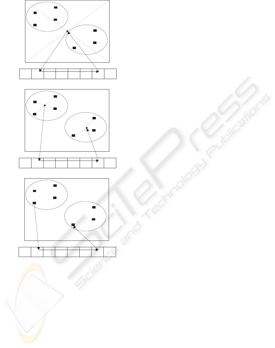
There are several ways to define the cost of the
movement between the feeder and a PCB, see Fig. 2.
At the end of every placement the arm has to return to
the feeder to pick up the next set of components. Af-
ter the arm has picked up these components it travels
back on the PCB. We can approximate the locations of
the arm on the PCB roughly using the centre of PCB
only (see Fig. 2 a). The second and more gentle way
to approximate the start and end positions of the pick-
up phase is to use the centre point of the locations
which belong to the same load of the arm (i.e. the set
of components simultaneously in the placement arm)
(Fig. 2 b). The third and the most accurate way is to
use the exact location of the last component of pre-
vious and the first component of the next placement
phase (Fig. 2 c). Note that the third method can only
be used if the actual order of the component place-
ments is known.
It is obvious that different pick-up orders w
o
for
the same w have in general different costs. Our aim is
to select, for a given w, a and s, the ordering (permu-
tation) w
o
of w with the minimal cost. Let us denote
this cost, which we call the cost of a pick-up event for
w (given a and s), with ecost(w, a, s).
Problem 1. (Single pick-up event problem, SPE)
Given w, a and s, compute ecost(w, a, s) and the as-
sociated pick-up sequence w
o
for w (supposing one
exists).
2.3 Cost of a Pick-up Sequence
The number of component placements per PCB is
normally very large in comparison to the total num-
ber of nozzles in arm. Therefore the placements
must be divided into several subjobs. Given a job
ICINCO 2007 - International Conference on Informatics in Control, Automation and Robotics
328
PCB
feeder
c
i-1
c
i-2
c
i-3
c
i-4
s(c)
i
c
i
c
i+2
c
i+1
PCB
feeder
c
i-1
c
i-2
c
i-3
c
i-4
s(c)
i
c
i
c
i+2
c
i+1
PCB
feeder
c
i-1
c
i-2
c
i-3
c
i-4
s(c)
i
c
i
c
i+2
c
i+1
s(c)
i+1
s(c)
i+2
s(c)
i+1
s(c)
i+2
s(c)
i+1
s(c)
i+2
(a)
(b)
(c)
Figure 2: Three different ways to define the cost of the arm
movement between the feeder and PCB.
w and an arm a, the pick-up sequence of w using a
is any partition of w into subjobs w
1
, w
2
, . . . , w
p
(i.e.
w = w
1
· w
2
···w
p
) such that a can pick up each w
i
(i = 1.. p). The length of such a pick-up sequence is p.
The cost of a pick-up sequence is simply the sum of
the costs ecost(w
i
, a, s) of individual pick-up events.
One can partition w into subjobs in many different
ways and the total picking cost depends on the par-
ticular partition. The minimum cost pick-up sequence
for given w, a and s is a pick-up sequence with a min-
imal cost denoted by mcost(w, a, s).
Problem 2. (Minimal pick-up sequence prob-
lem, MPS) Given w, a and s, find a pick-up sequence
w
1
, w
2
, . . . , w
p
for w such that
p
∑
i=1
ecost(w
i
, a, s)
is minimal and compute the associated mcost(w, a, s).
3 SOLVING THE SPE AND MPS
3.1 Pick-up Events
Let us first consider the SPE (problem 1) which deter-
mines for given w, a and s the minimal pick-up order-
ing w
o
. This problem can be solved for small a even
by a brute force -method which checks all the possi-
ble ways of feeder-to-nozzle-combinations. However,
for greater arm sizes the algorithm becomes soon un-
practical in special when the SPE-problem should be
solved repeatedly a great number of times.
We first consider only the movements above the
feeder unit and thus ignore the cost of moving to the
PCB and back. It is obvious that if w contains several
occurrences of the same component type, all of these
should be picked up once the arm is in the appropri-
ate location. (The is true, because the machine model
does not allow so called gang pick-ups) Hence, the
problem reduces into finding the shortest path con-
necting all the feeder locations
S(w) = {s(c) | c ∈ C(w)}.
Now let s
min
and s
max
be the minimal and maximal
elements of S(w). It is clear that the length of any
path connecting all the members of S(w) (points on
a line segment), is at least s
max
− s
min
. Therefore,
we have two obviously minimal connecting paths: the
ones connecting the points of S(w) in their increasing
or decreasing order.
In practise, the length of the initial movement de-
pends also on the location s(w
o
1
) and the initial lo-
cation of the arm (the location where it was left af-
ter placing the last component of the previous place-
ment). Similarly, the last pick-up is followed by the
movement to the first placement location on the PCB.
The placement order of w defines what these loca-
tions exactly are. If the placement orders of all pick-
up events w
1
, w
2
, . . . , w
p
are known beforehand, the
initial location of the arm, when event w
i
is started, is
the last placement of the previous event w
i−1
, and the
location we move after the pick-up of w
i
can be found
from the first placement of w
i
.
However, the placement order is not necessarily
known to us. Formerly the reason for this was that
MINIMIZING THE ARM MOVEMENTS OF A MULTI-HEAD GANTRY MACHINE
329
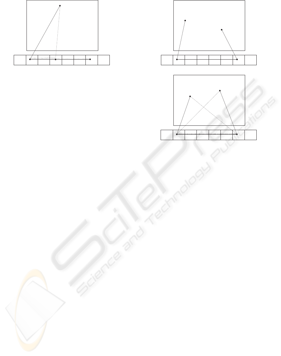
PCB
feeder
s
min
s
start
s
max
(x
c
,y)
c
Figure 3: The linear ordering of the pick-up points gives us
the minimal path.
the pick-up and the placement sequencing problems
were interconnected so that both of them should be
solved jointly. Currently, another reason for the lack
of this information has arisen: There are placement
machines which decide the printing order automati-
cally at the pick-up phase. The best we can then do is
to approximate the initial and final locations with the
center of the PCB or with the average of the place-
ment locations. In the former case, we use the same
constant location in all cost calculations, in the latter
case the center point is specific to each pick-up event.
Let us denote this center point with (x
c
, y
c
).
Consider the three pick-up points s
min
, s
max
and
s
start
, where s
start
is the first pick-up place. If
s
start
6∈ {s
min
, s
max
}, suppose (without loss of gen-
erality) that
s
start
− s
min
≤ s
max
− s
start
,
i.e. the start position is closer to the smallest posi-
tion than to the largest one. The minimal route on top
of the feeder goes now first from s
start
to s
min
(pick-
ing all the components on the way) and then all the
way to s
max
. The difference to the length of a route
starting directly at s
min
is hence s
start
− s
min
. Al-
though the distance from (x
c
, y
c
) to (s
start
, 0) might
be shorter than to (s
min
, 0), the difference is always
smaller than s
start
− s
min
due to the triangular in-
equality (consider the triangle with corners at (x
c
, y
c
),
(s
min
, 0), and (s
start
, 0)), see Fig. 3. Hence, the lin-
ear ordering of the points gives us the minimal path
even in this case. If the arm is moved by two motors,
one for the x-directional and one for the y-directional
movement and these operate at the same speeds, the
movement time is related to the maximum of the coor-
dinate distances (the Chebyshev distance). Naturally,
the triangular inequality holds here, too.
The SPE can now be solved trivially by
sorting the locations s(w
i
) into ascending or-
der. The smallest and largest positions are
then s(w
o
1
) and s(w
o
|w|
), respectively. The value
of ecost(w, a, s) is d((x
c
, y
c
), (s(w
o
1
), 0)) + s(w
o
|w|
) −
PCB
feeder
s
min
s
max
(x
i
,y)
i
(x
f
,y)
f
PCB
feeder
s
min
s
max
(x
i
,y)
i
(x
f
,y)
f
Figure 4: The arrangement of components depends on x
i
and x
f
.
s(w
o
1
) + d((s(w
o
|w|
), 0), (x
c
, y
c
)), where d is an appro-
priate metric. If the movements between the PCB and
the feeders are ignored (or the cost is constant) the
formula simplifies to s(w
o
|w|
) − s(w
o
1
).
Suppose now that the printing order is known, and
that (x
i
, y
i
) and (x
f
, y
f
) are the initial and final loca-
tion of the arm in some pick-up event. That is, (x
i
, y
i
)
is the location where the last component of the previ-
ous pick-up event was placed and (x
f
, y
f
) is the loca-
tion where the first component of this pick-up event
will be placed. A similar geometrical analysis gives
again (see Fig. 4), that
• if x
i
≤ x
f
, the component pick-ups should be ar-
ranged in an ascending order of s(c) and
• if x
i
> x
f
, the component pick-ups should be ar-
ranged in a descending order of s(c).
The corresponding value of ecost(w, a, s) is
then d((x
i
, y
i
), (s(w
o
1
)), 0)) + |s(w
o
|w|
) − s(w
o
1
))| +
d((s(w
o
|w|
), 0), (x
f
, y
f
)).
3.2 Pick-up Sequences
The task in the MPS is to partition a large w into sub-
jobs w
1
, w
2
, . . . , w
p
such that the accumulated pick-up
cost is minimal. Note first that the greedy partition-
ing that gives minimal number of pick-ups (Knuutila
et al., 2007) (pick up always as many components as
possible) does not always give an minimal solution
ICINCO 2007 - International Conference on Informatics in Control, Automation and Robotics
330

when the goal is to minimize the length of arm move-
ments. However, the greedy algorithm still minimizes
the number of pick-up rounds. Consider the following
example:
w = (c
1
, x
1
, y
1
), . . . , (c
5
, x
5
, y
5
),
s(c
1
) = 1, s(c
2
) = 2, s(c
3
) = 100,
s(c
4
) = 101, s(c
5
) = 102,
τ(c
i
) = τ for i = 1..5, and
a
max
= 3.
The greedy partitioning would first pick component
types c
1
, c
2
, c
3
and then c
4
, c
5
. The simplest defi-
nition of ecost(w, a, s) would give a cost of (100 −
1)+(102−101) = 100, whereas the cost for partition
c
1
, c
2
and c
3
, c
4
, c
5
would be (2− 1) + (102− 100) =
3.
The same counter example gives the following
costs for the second definition of ecost(w, a, s). In the
greedy case
d((x
c
, y
c
), (1, 0)) + (100− 1) +
d((x
c
, y
c
), (100, 0)) + d((x
c
, y
c
), (101, 0)) +
(102− 101) + d((x
c
, y
c
), (102, 0)),
and in the alternative case
d((x
c
, y
c
), (1, 0)) + (2− 1) +
d((x
c
, y
c
), (2, 0)) + d((x
c
, y
c
), (100, 0)) +
(102− 100) + d((x
c
, y
c
), (102, 0)).
Considering the geometry of the feeder (a straight line
segment), distances to adjacent slots from the PCB
center are practically the same. Hence, the greedy
distance is approximately
d((x
c
, y
c
), (1, 0)) + 3∗ d((x
c
, y
c
), (100, 0)) + 100,
and the alternative is
2∗ d((x
c
, y
c
), (1, 0)) + 2∗ d((x
c
, y
c
), (100, 0)) + 3.
If the distances to feeder slot 1 and slot 100 are ap-
proximately the same from the PCB center (e.g. they
are at the left and right ends of the feeder), then the al-
ternative partitioning is clearly a winner here, too. A
similar inspection can be carried out also for the third
definition of ecost(w, a, s).
3.2.1 Brute Force Method
Solving the MPS seems to lead to an exhaustive
search over all possible ways of partitioning w into
subsequences. Procedure
sequence
implements a
brute-force algorithm for this problem. The global
variables
best
and
bestcycle
store the value and the
partition of the best solution found so far. The cur-
rent partition is given by the array
cycle
. Argument
p
gives the level of a current recursive call and
cost
expresses the ecost of the subjobs 1 to (p-1). Algo-
rithm
sequence
is initially called as
sequence(1,0)
with
cycle[0] = 1
since at the first pick-up cycle
at least one component has to be picked up and the
cost should be zero before any components has been
picked up. At the beginning,
best
is initialized to
some large value. After the execution, the result is in
array
bestcycle
.
// cycle = array of the start indexes of
// pick-up cycles
// p = current pick-up cycle
// N = length of the placement sequence w
sequence (int p, int cost)
int i, k, x;
k := cycle[p - 1]; // start of the
// previous cycle
// i = tentative start of the next cycle
FOR i = k+1 TO k + pick-up head size DO
IF the pick-up head can pick components
from k to i - 1 THEN
x := ecost(k, i - 1);
IF ((cost + x) < best) THEN
IF i = N+1 THEN // solution
best := cost + x;
bestcycle := cycle;
ELSEIF i <= N
cycle[p] = i;
sequence(p + 1, cost + x);
END END END END
END
The greedy method to form a pick-up sequence
(introduced in (Knuutila et al., 2007)) minimizes the
number of pick-up-cycles for given w and a. The min-
imal solution (in terms of total length of arm move-
ments) found by
sequence
seems always to be clearly
better than that generated by the greedy method when
measuring the performance using the length of tour
the placing arm has to travel to pick up all components
for a certain job. A problem here is that
sequence
is
capable of solving only small problems in which the
job size is few dozens of components; its running time
explodes for placement tasks of practical size.
3.2.2 Dynamic Programming
We apply dynamic programming to search the mini-
mal solution in a fast way. Fast algorithm is required
also for this subproblem since searhing for a minimal
pick-up sequence will be an important part of higher
level optimization software. Consider job w of length
n. Dynamic programming can be applied since the
MINIMIZING THE ARM MOVEMENTS OF A MULTI-HEAD GANTRY MACHINE
331
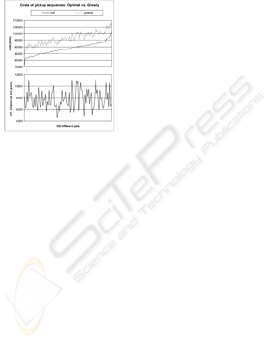
Figure 5: The pick-up sequence generated by the greedy
method is clearly worse than the minimal solution found by
exhaustive search when measuring the length of arm move-
ments in mm. We tested here 100 different jobs of length
600 with arm size of 20, 7 seven different nozzles, and 20
(also the number of feeders) different components per job.
solution for any suffix w
k
of job w must be mini-
mal regardless the solution of the earlier subjobs w
i
(i < k) which must be minimal, too. The minimal so-
lutions for all starting points of subjobs are searched
and memorized starting from the last one (the subjob
of length 1) and proceeding towards longer subjobs.
Finally, the minimal solution for the subjob of length
n (the actual job) is found. For this method the run-
ning time T(n, a
max
) is O(na
2
max
) in the worst case and
the memory usage M(n) = θ(n
2
).
Procedure
dynamic_sequence
uses global arrays
comp_costs
and
comp_parts
;
comp_parts
stores
the minimal cycle sequences for every suffix of a job
and
comp_costs
holds the costs of these sequences.
The procedure uses backward recursion by starting
from the end of the job and proceeding towards the
beginning. At each step
j
,
round_min
is set to some
big value and the maximum number of components
that the placing arm can hold simultaneously start-
ing from the
j
’th placement instruction is stored into
a_can
. Then, ecosts for all possible pick-ups of com-
ponents from
j
to (
j + a_can
) are calculated in turn
and summed with the costs of corresponding suffixes
stored in
comp_costs
. List
part_list
and variable
round_min
keep the information of the best cycle se-
quence of the current round.
Part_list
is formed
by linking the minimal cycle sequence list of a cor-
responding suffix on the right of the current one. Fi-
nally, the
bestcycle
(as in the previous algorithm) is
constructed on the basis of
comp_parts[1]
and the
minimal cost of the pick-up sequence for the job is
returned.
// bestcycle = array of the start indexes of
// the pick-up cycles for the
// minimal cycle sequence
// N = length of the placement sequence w
// part_list = linked list, integers as items
// comp_costs = array of minimum cost for all
// possible job suffixes
// starting positions
// between [1, N]
// comp_parts = array of length N of linked
// lists which items determine
// the minimums stored
// into comp_costs
dynamic_sequence : int
int i, j, x, round_min;
FOR j := N DOWNTO 1 DO
round_min := positive infinity;
a_can := max number of components
that arm can hold at once
starting from j’th placement
instruction;
FOR i := 1 TO a_can DO
x := ecost(j, j + i - 1);
IF j + i - 1 < N THEN
x := x + comp_costs[j + i];
END
IF x < round_min THEN
round_min := x;
create new part_list;
part_list.put_right(i);
IF j + i - 1 < N THEN
part_list.append(
comp_parts[j + i]);
END
END
END
comp_costs[j] := round_min;
comp_parts[j] := part_list;
END
construct bestcycle -table
by comp_parts[1] -list;
RETURN comp_costs[1];
END
The suffix of a job is independent of the prefix of the
job only in cases (a) and (c) of Fig. 2. Therefore, the
dynamic programming approach cannot be applied if
the placement locations are approximated as in case
(b). However, case (c) is sufficient; in practice the
component locations are usually known.
ICINCO 2007 - International Conference on Informatics in Control, Automation and Robotics
332
350
Feeder bankof20feeders
PCB
300
200
350
....................
50
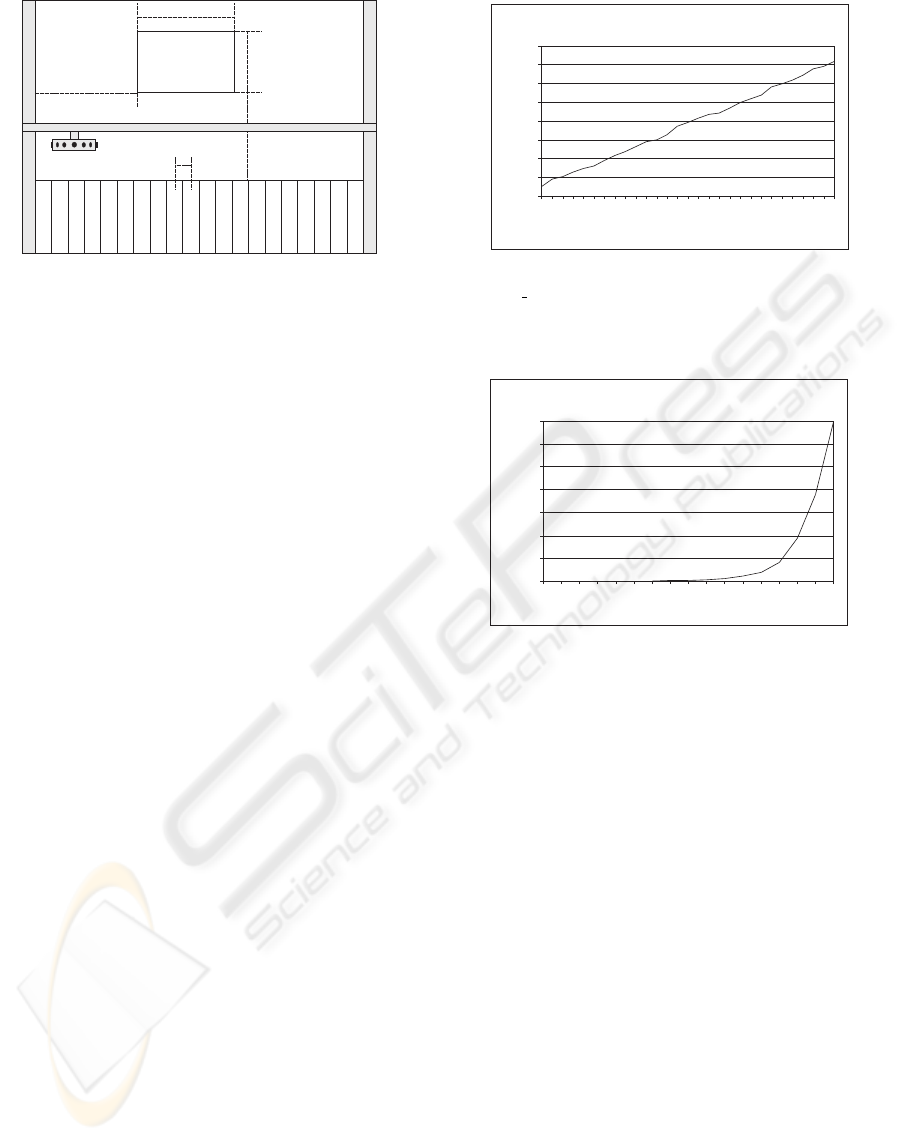
Figure 6: Some essential dimensions of a typical multi-head
gantry in mm. The distances are realistic and they represent
existing gantry-machines.
4 RESULTS OF EXPERIMENTAL
TESTS
In this section it is demonstrated that algorithm
dynamic_sequence
is fast enough to solve problems
appearing in practice. It is also experimented how the
cost of a pick-up sequence behaves when the arm size
varies. For evaluating procedure
dynamic_sequence
we use a Markov-model with 20 states to gen-
erate challenging component placement tasks, see
(Py
¨
otti
¨
al
¨
a et al., 2005) and (Py
¨
otti
¨
al
¨
a et al., 2006).
The model is fully connected and the transition prob-
abilities vary in wide range. As a result of this
data generation model, the component type of the ith
placement depends on the types of previous compo-
nents and the number of different component types
is non-uniform. However, the (x, y)-pairs (component
positions on a PCB) of placement instructions are still
uniformly distributed over the PCB in our test data
generator.
The dimensions of a the placement machine are
indicated in Fig. 6. Independent step motors move
the placement head in x- and y-directions with same
speed.
In all tests, the nozzles of a placing arm are se-
lected using the uniform distribution -based heuristic
introduced in (Py
¨
otti
¨
al
¨
a et al., 2006). In this heuristic,
different types of nozzles are chosen into the arm in
the same ratio as the nozzle type requirements occur
in the placement job. The running times are measured
in real-time seconds.
The average running times of the method of sec-
tion 3.2.2 for 100 jobs of each different length (job
length classes were 200, 300, 400,...,3000) are shown
in Fig. 7. The tests were performed for 20 different
component types, 7 nozzle types and arm size of 14.
The average running times show a clear linear ten-
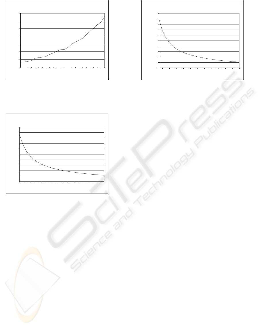
dency on the number of placements in the job. Figure
average running time
0
0,01
0,02
0,03
0,04
0,05
0,06
0,07
0,08
200
300
400
500
600
700
800
900
1000
1100
1200
1300
1400
1500
1600
1700
1800
1900
2000
2100
2200
2300
2400
2500
2600
2700
2800
2900
3000
job length
time (seconds)
Figure 7: The average running times of procedure
dynamic sequence.
for jobs of different length. The re-
sults are for each job length averages of N = 100 test jobs
generated by the Markov-model described earlier.
average running time
0
200
400
600
800
1000
1200
1400
10
11
12
13
14
15
16
17
18
19
20
21
22
23
24
25
26
job length
time (seconds)
Figure 8: The running times of brute force. -method for
jobs of different length.
9 shows how the running time of the method based on
dynamic programing changes when the arm capacity
is increased from 7 to 30. Again the running times
are averages of 100 different jobs for each arm size.
Job length was 600, the number of different compo-
nents 20, and the number of different nozzle types 7.
Note, that in both figures (7 and 9) the shape of the
curve correlates well to the complexity class of dy-
namic program. However, figure 8 shows that brute
force-based method cannot be used in practice.
Figure 10 demonstrates the decrease of the num-
ber of pick-ups when the arm size increases. Here the
numbers of pick-ups are the ones of minimal pick-
up sequences. The minimal cost of pick-up sequence
decreases notably when the number of nozzles in a
placing arm increases. Figure 11 shows this effect for
job length 600, component types 20, different nozzles
7, and 100 different jobs for every arm size between
7-30).
MINIMIZING THE ARM MOVEMENTS OF A MULTI-HEAD GANTRY MACHINE
333
average running time
0
0,01
0,02
0,03
0,04
0,05
0,06
0,07
7 8 9 10 11 12 13 14 15 16 17 18 19 20 21 22 23 24 25 26 27 28 29 30
arm size
time (seconds)
Figure 9: The average running times of varying arm sizes.
Averages are for N = 100 randomly generated jobs for each
arm sizes.
average number of pickups
0
50
100
150
200
250
300
350
400
450
500
7
8
9
10
11
12
13
14
15
16
17
18
19
20
21
22
23
24
25
26
27
28
29
30
arm size
number of pickups
Figure 10: The average number of pick-ups for varying arm
sizes.
5 CONCLUSION
In this research the subproblem relating to the control
of a multi-head gantry placing machine was consid-
ered. Unlike the usual approach to this topic, this arti-
cle focused on a situation where the placement order
of the components is fixed and the pick-up order of
the components was to be determined.
Multiple nozzles in the placement arm, the lin-
ear ordering of the different components in the feeder
unit, and the fact that different types of components
require different nozzles make this problem complex.
In this case, the greedy algorithm that minimizes the
number of component pick-ups does not, opposite
to expectations, yield the minimal length pick-up-
route of the placement arm. An efficient algorithm
that applies dynamic programming was developed for
searching the minimal pick-up sequence. The running
time of the algorithm is linear on the number of com-
ponents to be placed and quadratic on the arm size.
average cost of pickup sequence
0
50000
100000
150000
200000
250000
300000
350000
400000
450000
500000
7
8
9
10
11
12
13
14
15
16
17
18
19
20
21
22
23
24
25
26
27
28
29
30
arm size
cost (mm)
Figure 11: The average cost of pick-up sequences for vary-
ing arm sizes.
REFERENCES
Ayob, M., Cowling, P., and Kendall, G. (2002). Optimisa-
tion for surface mount placement machines. In Uni-
versity of Nottingham.
Ayob, M. and Kendall, G. (2005). A survey of surface
mount device placement machine optimisation: Ma-
chine classification. In Computer Science Technical
Report No. NOTTCS-TR-2005-8. University of Not-
tingham.
Ball, M. and Magazine, M. (1988). Sequencing of inser-
tions in printed circuit board assembly. In Operations
Research 36(2), pp. 192-201.
Crama, Y., Kolen, A., Oerlemans, A., and Spieksma, F.
(1990). Througput rate optimization in the automated
assembly of printed circuit boards. In Annals of OR,
Vol. 26, pp.455-480.
Knuutila, T., Py
¨
otti
¨
al
¨
a, S., and Nevalainen, O.S. (2007).
Minimizing the number of pickups on a multi-head
placement machine. In The Journal of the Operational
Research Society.
Kumar, R. and Li, H. (1995). Integer programming ap-
proach to printed circuit board assembly time opti-
mization. In IEEE Trans. Components, Packaging and
Manufacturing Technology, part B: Advanced Packag-
ing, Vol. 18 pp. 720-727.
Lee, S., Lee, H., and Park, T. (1999). A hierarchical method
to improve the productivity of a multi-head surface
mounting machine. In Proc. of the IEEE Interna-
tional conference on Robotics and Automation, De-
troit, Michigan.
Leip
¨
al
¨
a, T. and Nevalainen, O. (1989). Optimization of
the movements of a component placement machine.
In European Journal of Operational Research,38, pp.
167-177.
Py
¨
otti
¨
al
¨
a, S., Knuutila, T., Johnsson, M., and Nevalainen,
O.S. (2005). Improving the pickups of components on
a gantry-type placement machine. In TUCS Technical
Report 692. Turku Centre for Computer Science.
ICINCO 2007 - International Conference on Informatics in Control, Automation and Robotics
334

Py
¨
otti
¨
al
¨
a, S., Knuutila, T., and Nevalainen, O.S. (2006).
The selection of nozzles for minimizing the num-
ber of pick-ups on a multi-head placement machine.
In GTCM2006 Conference, Groningen, The Nether-
lands.
Sun, D., Lee, T., and Kim, K. (2004). Component allocation
and feeder arrangement for a dual-gantry multi-head
surface mounting placement tool. In International
Journal of Production Economics 95 (2005) 245-264.
MINIMIZING THE ARM MOVEMENTS OF A MULTI-HEAD GANTRY MACHINE
335
