TARGET VALUE PREDICTION FOR ONLINE OPTIMIZATION AT

ENGINE TEST BEDS

Alexander Sung, Andreas Zell

Wilhelm-Schickard-Institute for Computer Science, University of T

ubingen, Sand 1, T

ubingen, Germany

Florian Kl

opper, Alexander Vogel

Powertrain / Testing Methods, BMW Group, Munich, Germany

Keywords:

Online Optimization, Engine Test Bed.

Abstract:

The settling times of target functions play an important role in the domain of online optimization at the engine

test bed. Inert target functions generally induce long measuring times which lead to increased costs. In this

article, we analyze how previous knowledge about the physical behavior of target functions can be used to

early predict the ﬁnal steady state value to reduce measuring times.

1 INTRODUCTION

In recent years, model based algorithms have gained

signiﬁcance in the domain of online optimization

of combustion engines (Isermann, 2003). In this

area, known optimization systems like, for example,

Cameo (Gschweitl et al., 2001) and Vega (Breden-

beck, 1999) are in use, but the algorithm mbminimize

presented in (Kn

odler et al., 2003) (Kn

odler, 2004)

(Poland et al., 2003) also has found its place in real

applications.

An important and time consuming part of online

optimization is the extraction of measuring data at the

engine test bed. Inert target functions, like e.g. the

exhaust gas temperature, need a long time until the

ﬁnal steady state value of the target function – also

called target value – is reached for a certain combi-

nation of input parameters. In addition, the detec-

tion of the ﬁnal value is complicated by noise. On

the other hand, the behavior of transient oscillation is

often known, or can be derived from physical rules

in order to early predict the target value. This pro-

cedure is investigated in the given contribution, ﬁrst

in simulation and then on real engine data. Preced-

ing analysis like (Flohr, 2005) (Schropp, 2006) show

that the behavior of target functions in this application

domain can often be described by simple mathemat-

ical functions. A target value prediction during the

online optimization based on a small amount of data

therefore has the potential to reduce the effort of mea-

suring. The idea of prediction is not new, of course.

There is recent work like (Castillo and Melin, 2002)

(Han et al., 2004) (Teo et al., 2001) (Wang and Fu,

2005) which deals with this topic using approxima-

tors such as neural networks, genetic algorithms, or

support vector machines for predictions based on time

series.

2 TARGET VALUE PREDICTION

In this section, the algorithm of target value prediction

is presented on idealized, artiﬁcially composed mea-

suring data. In addition, the algorithm is tested with

regard to robustness against noise.

2.1 The Principle of Target Value

Prediction

The progression of target functions is often inversely

exponential. A typical example is the temperature. At

the engine test bed, the exhaust gas temperature is a

quantity, which reacts slowly to adjustments of the in-

put parameters in comparison with other quantities of

the engine. It is thereby an ideal candicate for the fol-

lowing analyses for two reasons: On the one hand, it

is easy to get a large amount of measuring data dur-

ing the time of transient oscillation due to the inertia

of the target function. On the other hand, the possible

108

Sung A., Zell A., Klöpper F. and Vogel A. (2007).

TARGET VALUE PREDICTION FOR ONLINE OPTIMIZATION AT ENGINE TEST BEDS.

In Proceedings of the Fourth International Conference on Informatics in Control, Automation and Robotics, pages 108-115

DOI: 10.5220/0001639301080115

 SciTePress

Figure 1: Idealized measuring data and the result of target

value prediction.

proﬁt of time gained by using target value prediction

is especially large.

Figure 1 shows artiﬁcially generated, idealized

measuring data of a target function with such a be-

havior, displayed by the black circles. The system is

steady at the beginning and reacts with a delay to the

adjustments of the input values. The recorded data

is used as basis for online calculations by the target

value prediction. With a function approximation al-

gorithm based on least squares optimization, the be-

havior of the target function is emulated, and a target

value is predicted. So, if the data is given as



f(x

)



with

f being the unknown target function, the objec-

tive is to ﬁnd parameter values~v = (v

) that ap-

proximate the error

E =

∑



· e

·x

+ v

−

f(x

)



→ min! (1)

best. The result for the idealized data is also shown

in ﬁgure 1. If the data is so ideal and free of noise

like this, an early determination of the target value is

simple. A greater challenge is given by the addition

of noise, which is shown in the next section.

An important aspect of the prediction lies in the

correct detection of the moment when the target func-

tion reacts to changes of the input. This point in time

is unknown in a real application, and the response

time often varies. In our applications, this moment

is determinated by a signiﬁcant change in the target

values over a longer span of time. Therefore, it is fun-

damental for our algorithm to have a continuous and

detailed record of the target function. Given the data



f(x

)



, we ﬁrst ﬁlter our plateaus by replacing ev-

ery set

i−n

,. . ., x

}|∀ j ∈ {1, . .., n} :

f(x

i− j

) =

f(x

)

with its ﬁnal data point x

discarding the rest, then we

choose the smallest x

from the set





f(x

i+δ

) −

f(x

)| > λ



max

f(x

) − min

f(x

)





δ and λ are empirically speciﬁed parameters.

During the online operation, the target value

prediction is updated constantly with additionally

recorded data. The algorithm is suited for online use,

because the calculation of the target value only re-

quires a few milliseconds. Depending on the noise,

the predicted target value often changes when new

measuring data is added, and the prediction improves

in quality with an increased amount of data. The qual-

ity of the target value prediction is compared to the

standard method, which is still in use at the test beds

at present. The standard method assumes that the tar-

get function is tuned after a ﬁxed amount of waiting

time, speciﬁed in advance. Then, an averaged mea-

suring value is used as ﬁnal target value. In our sim-

ulation the waiting time, also referred to as stationary

time, is set to the point in time when the target func-

tion has reached 95% of its ﬁnal value. At this point, a

measuring time of half the stationary time’s duration

is used. This is in accordance to the situation at the

engine test bed.

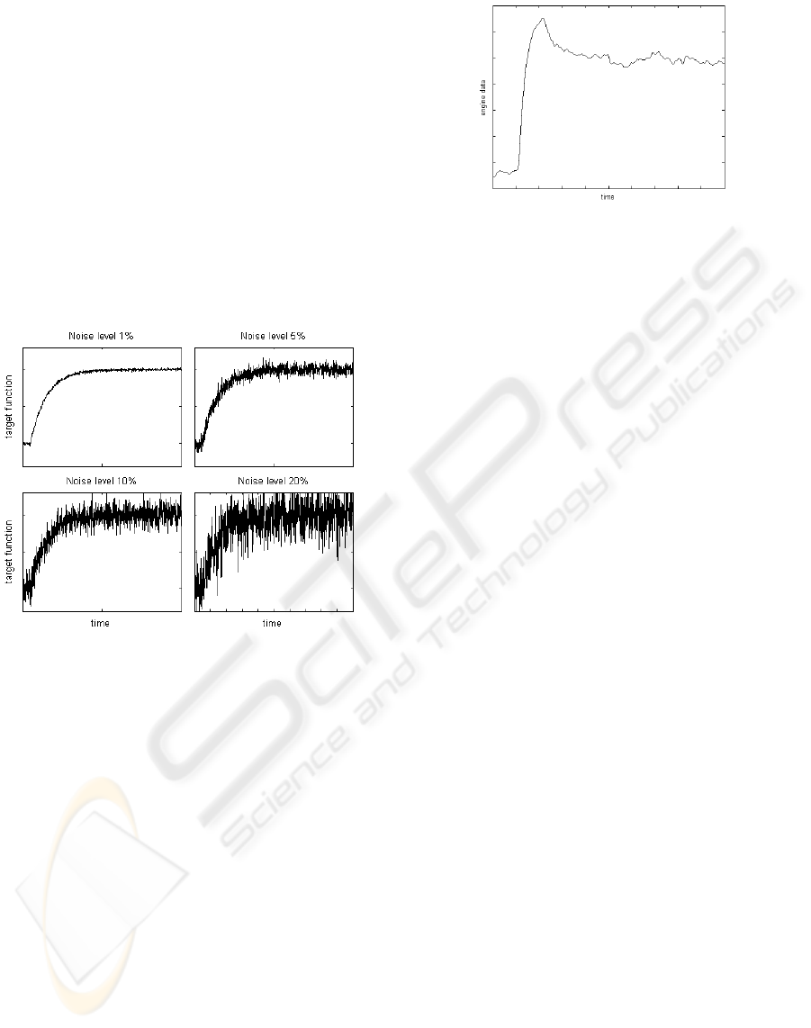
2.2 The Inpact of Noise

To test the robustness of the algorithm against noise,

the following tests were done. For different noise

levels 1000 test runs were evaluated each. Normal

distributed noise was used with a standard deviation

speciﬁed in relation to the range of the target values.

The results are the averaged saving of time in com-

parison to the standard method with a ﬁxed station-

ary time, as well as the relative error reduction ε, cal-

culated as the fraction of error ε

Ref

of the standard

method by which the prediction error ε

Pred

is lower,

and vice versa:

ε =

(

Ref

−ε

Pred

Ref

if ε

Pred

< ε

Ref

−ε

Pred

otherwise

. (2)

The higher the values are, the better target value pre-

diction worked. The prediction success displays how

often the prediction error was smaller than the error

of the standard method. The results are presented in

table 1.

Table 1: Investigation of noise inﬂuence.

Noise

Saving Error Prediction

level

of time reduction success

1% 46.1% 68.4% 96.6%

42.7% 42.6% 80.1%

39.3% 26.6% 68.4%

33.9% 7.5% 55.9%

10%

23.2% 0.0% 46.6%

By means of these results, it was possible to con-

ﬁrm the assumption that the function approximation

TARGET VALUE PREDICTION FOR ONLINE OPTIMIZATION AT ENGINE TEST BEDS

109

method of the target value prediction is able to deter-

mine the ﬁnal value more precisely than a simple av-

eraging after a ﬁxed stationary time. With increased

noise, which signiﬁcantly falsiﬁes the measuring data

especially in the early phase of transient oscillation,

the difference lessens because an early prediction is

not possible anymore in this case.

At a high noise level, which may commonly occur

in real applications, an early prediction is still possi-

ble, but the success is lacking. In the next section,

we show how this trade-off can be used to reduce the

overall measuring time of an optimization problem

without downgrading the ﬁnal results.

Figure 2 shows sample data sets with different

noise levels.

Figure 2: Sample data with different noise levels.

2.3 Addressing More Than Simple

E-functions

The simple E-function is only one of different pos-

sibilities to describe the behavior of target functions.

In our real application, for example, we found that a

twofold E-function v

· e

·x

+ v

· e

·x

+ v

was bet-

ter suited to describe the progression of the measuring

data. This and other unexpected behavior in the data

may be explained by the measuring technology, the

interplay of which still needs more investigations. In

this contribution, we want to mention two examples,

which occur commonly at the engine test bed.

Figure 3 shows an example of real engine data

with an overshooting behavior. In this case, the tar-

get values react to changes of the input parameters by

progressing past the ﬁnal steady state value ﬁrst, and

then continue retrogressive afterwards. The difﬁculty

lies in the fact that the overshooting behavior cannot

be detected before the retrogressive part is recorded.

Figure 3: An example of real engine data with overshooting

behavior.

An early target value prediction will therefore fail to

describe the progession correctly. For an optimiza-

tion problem with several measuring points, the deci-

sion whether to abort the measuring process due to an

early target value prediction can be made depending

on the signiﬁcance of the expected target value. For

example, if the current target value is already under

a certain threshold of importance and the predicted

value has even less impact on the optimization result,

a possible overshooting can be neglected.

Sometimes, a drift in the target values can be

detected. This behavior can be identiﬁed with tar-

get value predictions, too. If several predictions are

recorded over a longer period of time, it becomes ev-

ident that a small linear time is included in the under-

lying target function v

·e

·x

. In general,

however, the inﬂuence of drift at one single measuring

point is too small to have a signiﬁcant impact on the

ﬁnal steady state value. Since the detection of drift be-

havior is complicated by noise and requires a longer

period of measuring time, we neglect the possible oc-

currence of drift in general. This corresponds to the

standard measuring method, which determines the ﬁ-

nal result as an averaged measuring value.

3 RESULTS IN REAL

APPLICATIONS

This section consists of several applications from the

domains of both simulation and the engine test bed,

in which target value prediction improves the ﬁnal re-

sults.

3.1 Model-based Optimization

In the applications of this section, we used a model-

based approach for the optimization of the input pa-

rameters of a target function that was deﬁned over a

given input space. The models of the target function

were generated by a committee of neural networks

ICINCO 2007 - International Conference on Informatics in Control, Automation and Robotics

110

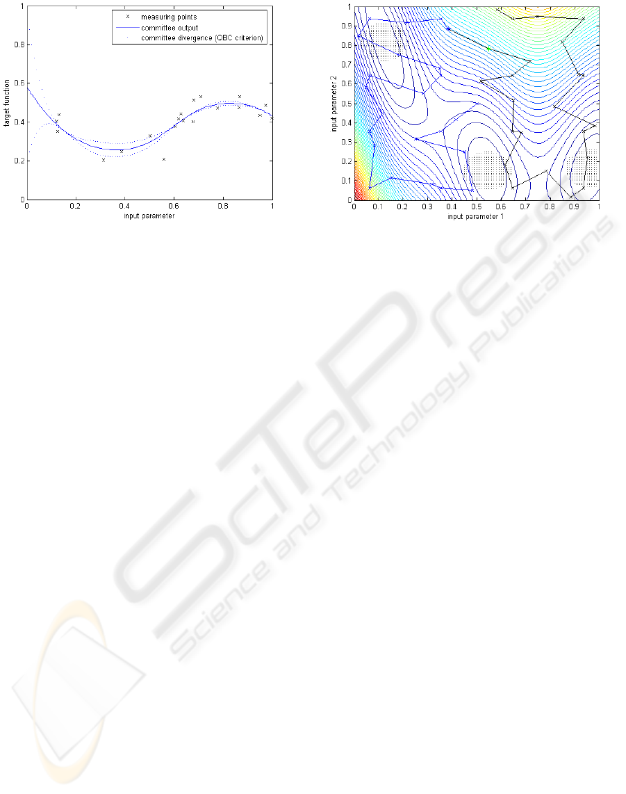
Figure 4: Model output of a committee of neural networks

and linear regression. The QBC criterion is a measurement

for the uncertainty and supplies the largest values to the

points where the committee’s individual models diverge the

most.

and LLR models, the output of the later being a lin-

ear combination of non-linear basic functions. Neural

networks have been long established in model-based

optimization, as illustrated in (Hafner, 2002) (Hafner

et al., 2000) (Sch

uler et al., 2000), for example. The

strengths of neural networks for our use lies in the

ability to produce a good overall approximation of the

target function based on few data points without prior

knowledge. The LLR models, on the other hand, are

designed to speciﬁcally describe local behavior in the

input space in detail.

Based on such a model, we calculate a QBC crite-

rion (query by committee), of which ﬁgure 4 provides

an example over an one-dimensional input space. The

QBC criterion supplies the largest values to the points

where the committee’s individual models diverge the

most. The information of already known measuring

points is included to avoid repeated measuring at the

same input values. The expression ”query” here de-

notes the decision-making process to determine the

next measuring point with the aid of the currently

available model. This method will be used in the fol-

lowing subsection.

3.2 Optimization in a Simulation

Environment

As a ﬁrst application, we used our algorithm in a

simulation environment, which was designed for the

optimization of an engine model. Measuring points

were chosen in a two-dimensional search space by a

D-optimal DoE-method (R

opke, 2005) (Weber et al.,

2005). The goal was to ﬁnd the local minima and

to model the regions around them with the least er-

ror possible. We used the Branin function as the tar-

Figure 5: Snapshot of the online optimization in a simula-

tion environment. The black dots mark the test error set.

get function and simulated it to be inert, according to

what was described in the section before. Note, that

the test set consisted of test points near the local min-

ima only, in order to display the optimization goal.

Figure 5 shows the setup of the experiments. Our al-

gorithm was tested against the standard method with

ﬁxed stationary and measuring time.

There are two conditions, after which the predic-

tion based algorithm completes the measuring process

at a speciﬁc measuring point and evaluates the gath-

ered measuring data via prediction: In the standard

case, analogous to the section before, the measuring

process is ﬁnished when the predicted value is stable

over a certain period of time. This is calculated with

the term



mean



p(t −δ), .. . , p(t − 1)



− p(t)



< α

∧ std



p(t −δ), .. . , p(t − 1)



< α (3)

using the predicted values p(t) after normalization.

The parameters δ = 30 (seconds) and α = 0.01 are

empirically determined based on real engine data.

In addition, however, there is a possibility to abort

the measuring when the expected target value is too

high to be a local minimum. In this case, the value

predicted at that moment is used as an estimated tar-

get value, even if it is to be expected that the error at

this point is quite large. The intention of this method

is to save measuring time at unimportant measuring

points to gain a ﬁrst rough engine model und use the

saved time to explore the regions of minima in detail.

Figure 6 shows two cases where the measuring pro-

cess was completed due to early predictions. In the

ﬁrst case, the measuring was complete since the pre-

dicted values leveled off at the point in time marked

by the dotted line. The second case shows an exam-

ple where the expected value was considered irrele-

vant for the minimization problem. The measuring

process was aborted in this case.

TARGET VALUE PREDICTION FOR ONLINE OPTIMIZATION AT ENGINE TEST BEDS

111

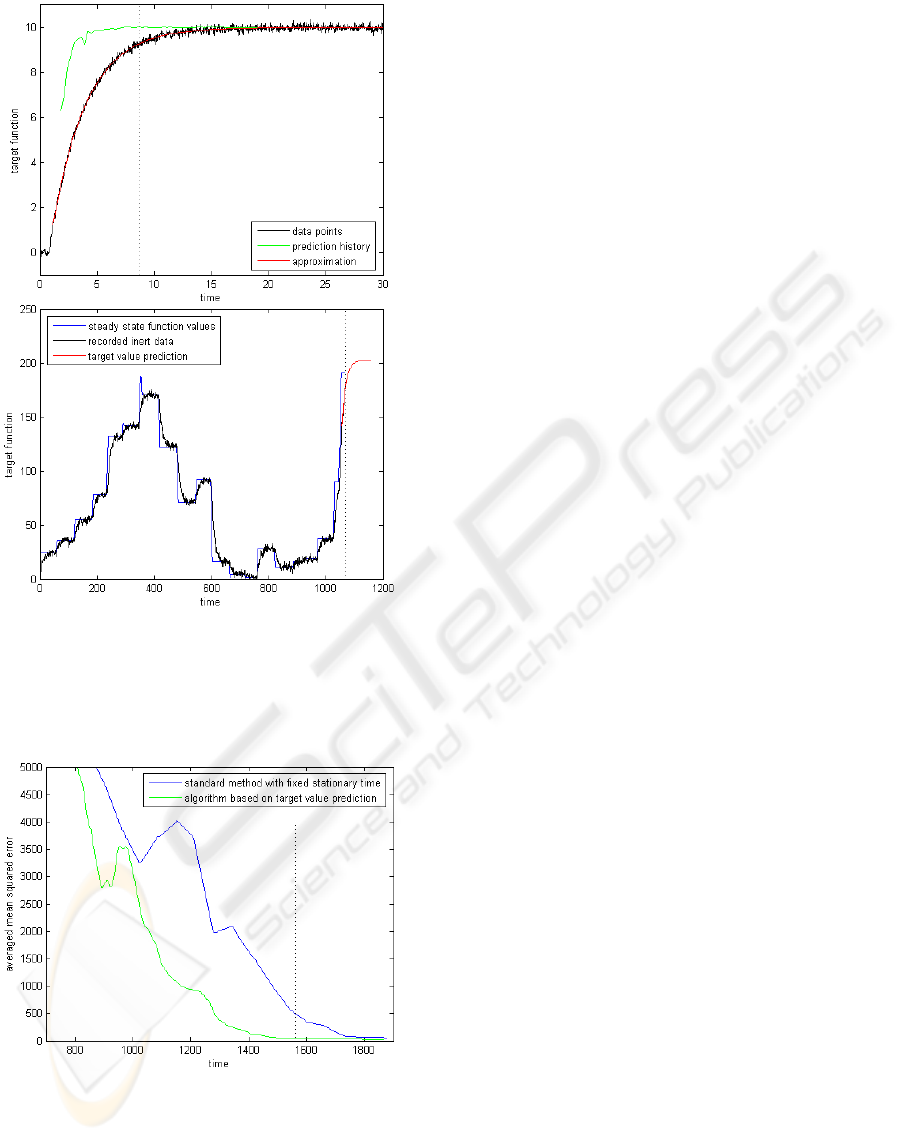
Figure 6: Examples of measuring processes completed due

to the evaluations of predicted values. In the ﬁrst example,

the prediction is considered reliable, in the second exam-

ple, the expected value is considered umimportant for the

optimization.

Figure 7: Test error progression of the online optimiza-

tion in a simulation environment. The standard method is

displayed in blue, the target value prediction algorithm is

shown in green. The dotted line shows when the target value

prediction algorithm completed the initial set of data points.

Two additional rules proved to be useful for the

optimization. Measurings with target values near the

expected optimum will not be aborted, and measur-

ings near local minima based on the current, incom-

plete model will also not be aborted. The thresholds

for these options are set by the user based on rough

previous knowledge at this time, but they are not sen-

sitive. These rules grant an additional certainty that

no information will be lost unnecessarily.

Figure 7 shows the progression of the test error

during the optimization over time, as an average over

72 test runs. After 74.4% of the time that the standard

method needed in total, the target value prediction al-

gorithm evaluated the initial set of measuring points.

At that point, our algorithm created a function model

with a test error of 41.6, while the model of the stan-

dard method still had a test error of 502.6. The reason

for this huge difference lies in the fact that the stan-

dard method did not yet deal with several measuring

points, so the error near those is still very large, of

course. The ﬁnal test error of the standard method

was 31.4.

In addition to the initial set of measuring points,

the prediction based algorithm used the saved time

to measure additional data points. To generate these

points, the current model of the target function was

used to locate the regions near local minima, as ex-

plained in the subsection before. Based on QBC cri-

terion, the additional measuring points were chosen

by a line search algorithm. With the additional data

points, the ﬁnal test error could be reduced to 17.7

with a 43.6% improvement in comparison with the

standard method.

In this scenario, our algorithm was able to produce

a rough interim result in a shorter time. On the other

hand, using the complete amount of time available,

our algorithm was able to improve the ﬁnal results in

comparison with the standard method.

3.3 Target Value Prediction on Real

Engine Data

As an example with real application data, the target

value prediction algorithm was used on engine data,

which was provided by the BMW Group in Munich.

The data consists of exhaust gas measurings and de-

scribe load step responses. The range of values has

been scaled to make the relative error values compa-

rable. The results contain 126 data sets.

Dealing with real engine data poses a problem,

which makes a presentation of the results according

to simulation difﬁcult: The real ﬁnal values of the

target function are unknown. Even after measuring

for minutes, it is possible that the transient oscillation

of several target functions still have not ﬁnished. An

open-ended measuring is not viable, however. Figure

ICINCO 2007 - International Conference on Informatics in Control, Automation and Robotics

112

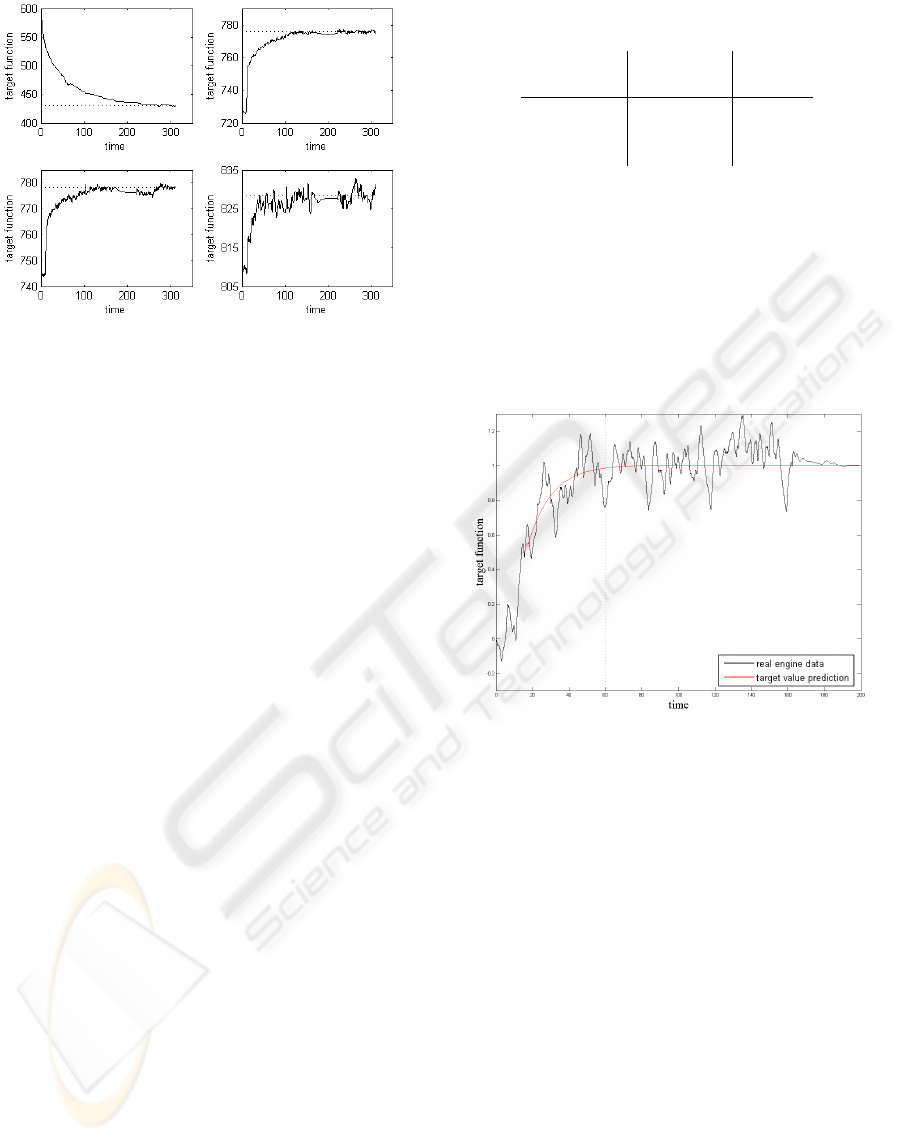
Figure 8: Examples of recorded engine data, which still

have not reached their ﬁnal values at the end of the record-

ing. The plateaus are a phenomenon of the measuring tech-

nology at the engine test bed. For comparison, the predicted

target value is included as a dotted line.

8 shows several examples of recorded engine data,

which still have not reached their ﬁnal values at the

end of the recording. Plateaus in the recorded data

arise because the measuring process is disabled dur-

ing the time of evaluating and saving the engine data

at the engine test bed. The data points after this point

in time still vary, however. Therefore, additional as-

sumptions, which are derived from the simulation, are

made for the following data evaluations.

In the practice of test bed operations, target func-

tions are assumed to have reached their ﬁnal values

after a certain amount of stationary time. A conclus-

ing averaged value is then accepted as target value.

In the given data, the stationary time has been set to

60 seconds. Afterwards, a measuring has been per-

formed over a timespan of 30 seconds, after which

the averaged value has been calculated. This value

was used for comparisons to rate the target value pre-

diction algorithm. The results from simulation show

that with an appropriate modeling of the target func-

tion progression given, the target value can be esti-

mated more precisely by a corresponding prediction

than by an averaged measuring value. For this reason

we assume that, in the case of real engine data, the

predicted target value, which was calculated based on

all available measuring data, approximates the real ﬁ-

nal value best. The examples in ﬁgure 8 include the

ﬁnal predicted target value for comparison. With re-

gard to this value, the results can be illustrated as in

table 2.

In the ﬁrst column, a maximum error level is

given. The second column shows in how many cases

this error level was reached. The error level was

reached when the difference of the prediction result

to the expected ﬁnal value did not exceed the given

Table 2: Evaluation of error levels using target value pre-

diction.

Maximum

Threshold Saving

error

success of time

3% 14.3% 21.4%

27.0% 25.1%

10%

63.5% 38.4%

level for at least 10 seconds. The difference is again

calculated in relation to the range of the target func-

tion. In the last column, the averaged amount of time

is shown that could be saved in those cases where the

error level was reached. The results for the compari-

son with the standard method in analogy to simulation

are a saving of time of 26.4% and an error reduction

of 3.3%. The prediction thereby gave a better result

in 52.4% of the tests.

Figure 9: Successful target value prediction (red line) ap-

plied on real engine data (black line). Only the ﬁrst part on

the left side of the dotted line was used for the prediction.

The real target value progression is shown for comparison.

Figure 9 shows an exemplary and successful target

value prediction based on engine data. In this case, a

similarity to the simulated E-function is identiﬁcable.

The complete engine data is drawn in black, while the

green dashed line highlights what data was available

to the prediction algorithm. The predicted behavior is

shown in red.

3.4 Model-based Optimization of a

Combustion Engine

As another application, we modeled a target function

of an engine over a two-dimensional parameter space.

The problem we had hereby was that there was not

enough real engine data available for an additional

large, independet test set. So, to evaluate the algo-

rithms on the real application, we had to create a sim-

ulated reference. We did this by creating an engine

TARGET VALUE PREDICTION FOR ONLINE OPTIMIZATION AT ENGINE TEST BEDS

113

model with the given engine data. This served as a

basis for calculations about test errors.

In analogy to the subsection before, we wanted

to explore the input space by measuring certain data

points. The target values were real engine data, and

therefore the measuring process was inert. With the

acquired data, a model was created both for our algo-

rithm based on target value prediction as well as for

the standard method using stationary and measuring

times. The goal was to ﬁnd the local minima with a

good representation of their immediate environments.

Note that we are refering to three different models

now. The ﬁrst one is created with steady state val-

ues and serves as reference. The other two models

are calculated during the optimization process where

recorded engine data on the inert target function is

evaluated. Figure 10 shows the ﬁrst of these models

which represents the engine’s target function in steady

states. Another fourth model is created by using tar-

get value prediction without the goal to minimize op-

timization time, but to achieve best test error values

instead.

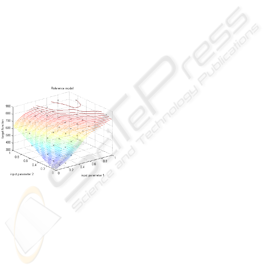
Figure 10: Model of the target function based on real engine

data, and the real measuring data. The function values from

this model are used as reference in our tests.

The measuring process consisted of approach-

ing and measuring 38 data points. Using the stan-

dard method, the ﬁnal mean squared error was 231.1.

The algorithm using target value prediction was able

to reach an error of 147.4 after 75.2% of the time

which the standard method needed, an improvement

of 36.8% in comparison to the standard method.

Therefore, the target value prediction could be used

to save time to early generate an engine model that

had a lower test error based on the reference model.

Furthermore, the predictions can also be done using

the same amount of time which the standard method

uses. In this variation the ﬁnal result was 139.3, an

improvement of 39.7%.

4 CONCLUSION AND

PROSPECTS

In this article we described the idea and methodology

of target value prediction. Thereby, the fundamental

assumption was that the behavior of the target func-

tion after adjusting the input parameters can be de-

scribed with inversely exponential E-functions. Re-

sults from both simulation and practice show the pos-

sible success of this algorithm. We demonstrated that

the strength of the target value prediction does not lie

in single measurings, since there is always some sort

of trade-off between saving of time and precision loss

included. Given a larger scope of an entire optimiza-

tion problem, however, exactly this trade-off can be

used to concentrate available resources to the impor-

tant parts of the problem and to save valuable time at

less signiﬁcant aspects.

Due to the nature of the prediction method to de-

tect the important regions of an optimization prob-

lem, we expect the algorithm to scale well with larger

problems where the areas of solutions do not scale ac-

cordingly at all. Further work will apply the proposed

method to other problems in the domain of online op-

timization and continue to show its capacity.

REFERENCES

Bredenbeck, J. (1999). Statistische Versuchsplanung

ur die Online-Optimierung von Verbrennungs-

motoren. In MTZ-Motortechnische Zeitschrift und

MTZ-Worldwide, 60 (11). MTZ Press.

Castillo, O. and Melin, P. (2002). Hybrid intelligent sys-

tems for time series prediction using neural networks,

fuzzy logic, and fractal theory. In IEEE Transactions

on Neural Networks, 13 no. 6, pages 1395–1408.

Flohr, A. (2005). Konzept und Umsetzung einer Online-

Messdatendiagnose an Motorpr

ufst

anden. PhD the-

sis, University of Technology Darmstadt.

Gschweitl, K., Pﬂuegl, H., Fortuna, T., and Leith-

goeb, R. (2001). Steigerung der Efﬁzienz in

der modellbasierten Motorenapplikation durch die

neue CAMEO Online DoE-Toolbox. In ATZ-

Automobiltechnische Zeitschrift und ATZ-Worldwide,

page 103 (7/8). MTZ Press.

Hafner, M. (2002). Modellbasierte station

are und dynami-

sche Optimierung von Verbrennungsmotoren am Mo-

torenpr

ufstand unter Verwendung neuronaler Netze.

PhD thesis, University of Technology Darmstadt.

Hafner, M., Sch

uler, M., and Isermann, R. (2000). Ein-

satz schneller neuronaler Netze zur modellbasierten

Optimierung von Verbrennungsmotoren - Teil 2: Sta-

tion

are und dynamische Optimierung von Verbrauch

und Emissionen. In Motortechnische Zeitschrift

(MTZ), 61 no. 11. MTZ Press.

ICINCO 2007 - International Conference on Informatics in Control, Automation and Robotics

114

Han, M., Xi, J., Xu, S., and Yin, F.-L. (2004). Prediction

of chaotic time series based on the recurrent predic-

tor neural network. In IEEE Transactions on Signal

Processing, 52 no. 12, pages 3409–3416.

Isermann, R. (2003). Modellgest

utzte Steuerung, Regelung

und Diagnose von Verbrennungsmotoren. Springer-

Verlag.

odler, K. (2004). Methoden der restringierten Online-

Optimierung zur Basisapplikation moderner Verbren-

nungsmotoren. PhD thesis, University of T

ubingen.

odler, K., Poland, J., Zell, A., Fleischhauer, T., Mitterer,

A., and Ullmann, S. (2003). Model-based online opti-

mization of modern internal combustion engines, part

2: Limits of the feasible search space. In MTZ World-

wide (Motortechnische Zeitschrift), 64 no. 6, pages

30–32, German edition 520–526. MTZ Press.

Poland, J., Kn

odler, K., Zell, A., Fleischhauer, T., Mitterer,

A., and Ullmann, S. (2003). Model-based online opti-

mization of modern internal combustion engines, part

1: Active learning. In MTZ Worldwide (Motortech-

nische Zeitschrift), 64 no. 5, pages 31–33, (German

edition: 432–437). MTZ Press.

opke, K. (2005). DoE – Design of Experiments. In Meth-

oden und Anwendungen in der Motorenentwicklung.

verlag moderne industrie.

Schropp, S. (2006). Optimization of measurement data log-

ging at engine test benches. Master’s thesis, Univer-

sity of Technology Munich.

Sch

uler, M., Hafner, M., and Isermann, R. (2000). Einsatz

schneller neuronaler Netze zur modellbasierten Op-

timierung von Verbrennungsmotoren - Teil 1: Mod-

ellbildung des Motor- und Abgasverhaltens. In Mo-

tortechnische Zeitschrift (MTZ), 61 no. 10. MTZ

Press.

Teo, K. K., Wang, L., and Lin, Z. (2001). Wavelet packet

multi-layer perceptron for chaotic time series predic-

tion: Effects of weight initialization. In Lecture Notes

in Computer Science, Vol. 2074, pages 310–317.

Wang, L. and Fu, X. (2005). Data mining with computa-

tional intelligence. In IEEE Transactions on Neural

Networks, 17 no. 3. Springer.

Weber, M., K

otter, H., Schreiber, A., and Isermann, R.

(2005). Model-based Design of Experiments for Static

and Dynamic Measurements of Combustion Engines.

In 3. Tagung: Design of Experiments (DoE) in der

Motorenentwicklung, Berlin.

TARGET VALUE PREDICTION FOR ONLINE OPTIMIZATION AT ENGINE TEST BEDS

115