
SLIDING MODE CONTROL FOR HAMMERSTEIN MODEL BASED
ON MPC
Zhiyu Xi and Tim Hesketh
School of Electrical Engineering & Telecommunications
University of New South Wales
Australia
Keywords:
Sliding mode, reaching control, equivalent control, MPC, Hammerstein model, nonlinearity.
Abstract:
This paper addresses discrete sliding mode control of nonlinear systems. The nonlinear system is identified
as a Hammerstein model firstly to isolate the nonlinearity from the sliding surface design. An MPC law
is employed to design the sliding surface. Then Utkins method of equivalent control is used. The method
illustrates the effect of the nonlinearity on reaching control. The ball and beam system is adopted as an
example. Simulation and on-line results are provided.
1 INTRODUCTION
Variable structure systems (VSS) have been exten-
sively used for control of dynamic industrial pro-
cesses. The essence of variable structure control
(VSC) (Raymond et al., 1988) is to use a high
speed switching control scheme to drive the nonlin-
ear plant’s state trajectory onto a specified and user
chosen surface in the state space which is commonly
called the sliding surface or switching surface, and
then to keep the plant’s state trajectory moving along
this surface. The surface is chosen to produce spec-
ified dynamic behaviour. Once the state trajectory
intercepts the sliding surface, it remains on the sur-
face for all subsequent time, sliding along the sur-
face, leading to the term “sliding mode”. Sliding
mode controller design comprises two stages. The
first is the design of sliding surface, while the second
forces the state to approach the sliding surface from
any other region of the state space, and remain on it.
The ball and beam system is a widely used lab-
oratory process. It reflects typical control problems
which include a double integrating factor, nonlinear-
ity, time delay and noise. In the ball and beam sys-
tem, a conductive ball lies on the beam comprised
of two parallel rods, and is free to roll along the
beam. A resistive strip, with impedance proportional
to length, covers one of the rods. The other rod is con-
ductive. The position of the ball can be determined
by introducing a small current through the rods and
measuring the resulting voltage, which varies with
impedance as the ball moves. One end of the beam
is fixed and the other is mounted on the output shaft
of a DC servo motor so the beam is tilted as the motor
shaft rotates. The control task is to regulate the posi-
tion of the ball by altering the angular shaft position
of the DC motor.
Design from an identified model has potential ad-
vantages in nonlinear control for the ball and beam,
and more generally. It relies on mathematical tools
and algorithms that build dynamical models from
measured data. Relatively simple structures of non-
linearity may be used to describe complex nonlinear
systems or ones for which models are difficult to de-
rive. In this paper, discrete sliding mode control of a
system described by a Hammerstein model will be ad-
dressed. This provides a simple method to deal with
nonlinear systems using VSC. The ball and beam sys-
tem will be used as an example to illustrate the design
procedure.
The control of a Hammerstein model has been ad-
dressed in the past by several authors (cite15,cite16).
Satisfying performance has been derived. In (Hwang
and Hsu), Hwang and Hsu talked about nonlinear con-
trol profile based on Hammerstein model in case of
model uncertainty. They also introduced an inverse
block into the system. Meanwhile, they spent a lot
effort on designing an observer.
232
Xi Z. and Hesketh T. (2007).
SLIDING MODE CONTROL FOR HAMMERSTEIN MODEL BASED ON MPC.
In Proceedings of the Fourth International Conference on Informatics in Control, Automation and Robotics, pages 232-237
DOI: 10.5220/0001639402320237
Copyright
c
SciTePress

2 HAMMERSTEIN MODEL
Hammerstein models are amongst those most com-
monly used for nonlinear identification. They are ca-
pable of providing simple nonlinear models for a wide
range of engineering problems. The model is charac-
terized by a static nonlinearity followed by a linear
time invariant (LTI) block. A typical Hammerstein
model for a process is shown in Figure 1:
n
u x +
+
y
Nonlinear
Static
Linear
Dynamic
Figure 1: Typical Hammerstein model.
y(t) = Tx(t) + n(t) (1)
x(t) = f(u(t)) (2)
where x(t) and y(t) are the inputs and outputs respec-
tively, n(t) is additive noise, f is the nonlinear map-
ping, T is the transfer function of linear part which
can be written as
T =
b
0
+ b
1
q
−1
+ b
2
q
−2
+ ··· + b
m
q
−m
1+ a
1
q
−1
+ a
2
q
−2
+ ··· + a
n
q
−n
with q
−1
representing the unit delay operator.
In this way, the nonlinearity of system is separated
from the linear block. This leads to the possibility of
ignoring the nonlinearity during key steps in the con-
troller design. Also, the nonlinear block in the Ham-
merstein model is a polynomial, which is a relatively
simple form. This reduces problems introduced by
complex nonlinearities such as exponentials and si-
nusoids.
3 DISCRETE SLIDING MODE
CONTROL DESIGN
3.1 Sliding Surface Design
Suppose the state space model of the above Hammer-
stein model is:
z(t) = Az(t − 1) + Bx(t) (3)
y(t) = Cz(t) + ¯n(t) (4)
where x(t) = f(u(t)).
Performing a similarity transformation defined by
an orthogonal matrix P:
z
l
= Pz = [z
1
: z
2
]
T
, A
l
= PAP
T
, B
l
= PB =
0
B
2
,
(5)
where z
1
does not have direct dependence on the in-
put nonlinearity. Sliding surface design may be un-
dertaken considering only z
1
, treating z
2
as an “input”
to the partitioned equations. In this way, the nonlin-
earity may be ignored while determining the sliding
surface, which is linear.
The partitioned state equations corresponding to
(3) and (4) may now be expressed in the following
way:
z
l1
(t +1) = A
l11
z
l1
(t) + A
l12
z
l2
(t) (6)
z
l2
(t +1) = A
l21
z
l1
(t) + A
l22
z
l2
(t) + B
l2
x(t).(7)
Suppose
sz
l
(t) = [
s
1
s
2
··· s
v
]z
l
(t) = w
1
z
l1
(t)+w
2
z
l2
(t)
in which v is the dimension of the corresponding state
vector, and s is the sliding surface, then the sliding
condition is
w
1
z
l1
(t) + w
2
z
l2
(t) = 0,
which yields
z
l2
(t) = −w
−1
2
w
1
z
l1
(t). (8)
Substitute (8) into (6) then we have,
z
l1
(t + 1) = A
l11
z
l1
(t) − A
l12
w
−1
2
w
1
z
l1
(t) (9)
= (A
l11
− A
l12
w
−1
2
w
1
)z
l1
(t). (10)
Any standard design algorithm which produces a
linear state feedback controller for a linear dynamic
system can be used to determine (A
l11
− A
l12
w
−1
2
w
1
)
and achieve desired performance through selection
of sliding mode dynamics (Spurgeon, 1992). Pole
placement is an obvious way of assigning closed
loop eigenvalues, but for systems of higher order the
method has attendant difficulties.
MPC is a widely-used method for calculating
closed-loop feedback controller gains. It is suitable
for systems with high order. It is employed to de-
termine the sliding surface in this paper. Consider-
ing z
l1
(t + 1) = A
l11
z
l1
(t) + A
l12
z
l2
(t), z
l2
(t) can be
viewed as the input to a new system the state vector
of which is z
l1
(t). An MPC criterion minimizes the
cost function which is defined to be:
J =M
⊤
t+1
M
t+1
+λU
⊤
t
U
t
. (11)
where
M
t+1
=
z
l1
(t +1)
z
l1
(t +2)
···
z
l1
(t + N)
,U
t
=
z
l2
(t)
z
l2
(t +1)
···
z
l2
(t +N − 1)
.
The goal is to fix the relationship between z
l2
(t) and
z
l1
(t) to prescribe desirable performance for the nom-
inal sliding mode dynamics. The controller gain de-
rived is:
z
l2
(t) = −kz
l1
(t) (12)
SLIDING MODE CONTROL FOR HAMMERSTEIN MODEL BASED ON MPC
233

which means that
σ(z
l
(t)) =
h
k
.
.
. I
i
z
l
(t) (13)
Note that inversion of the similarity transforma-
tion (using P) is needed to recover z(t) from z
l
(t).
Then sz(t) is the sliding surface.
3.2 Sliding Mode Controller Design
The reaching law still applies for discrete systems.
However, the state trajectory may overshoot the slid-
ing surface repeatedly, so that true sliding does not
occur. The switching manifold of a discrete VSC sys-
tem is called an ideal switching manifold because in
all practical situations, switching seldom occurs on
it. The size of each successive overshoot is non-
increasing and the trajectory stays within a specified
band which is called a
quasi-sliding mode
(QSM).
The specified band is called
quasi-sliding mode band
(QSMB) (Gao et al., 1995) and is defined by
{
x | −∆ < s(x) < ∆
}
(14)
where 2∆ is the width of the band.
Consider the single input linear system with
switching manifold s, a common type of sliding mode
controller is:
u(t) = u
eq
(t) + u
2
(t) (15)
where u
eq
(t) represents the equivalent control which
ensures sliding and u
2
(t) drives the state onto the slid-
ing surface, (termed reaching control).
According to the definition of sliding mode, we
have
σ(t +1) = sz(t+1) = sAz(t)+sBu
eq
(t) = σ(t). (16)
and
σ(t) = 0.
From the above, the equivalent control can be de-
scribed as follows:
u
eq
(t) = −(sB)
−1
sAz(t). (17)
Then let us consider the reaching control law. For
continuous SMC problem, a simple Lyapunov func-
tion V(σ(z)) = 0.5σ
T
(z)σ(z) is considered. The cor-
responding reaching condition is
∂V
∂t
= σ
T
·
σ < 0. (18)
In discrete system design, the equivalent form of this
condition is
[σ(t + 1) − σ(t)]σ(t) < 0. (19)
Substitute (3), (4), (15) and (17) into (19) then:
[σ(t + 1) − σ(t)]σ(t) = (sAz(t) + sBu(t) − sz(t))sz(t)
= ((sB)((sB)
−1
sAz(t)
+u(t)) − sz(t))sz(t)
= (sB(u(t) − u
eq
(t))
−sz(t))sz(t).
= (sBu
2
(t) − sz(t))sz(t).
u
2
(t) should be selected to ensure that:
sBu
2
(t) < sz(t) when sz(t) > 0 (20)
sBu
2
(t) > sz(t) when sz(t) < 0. (21)
As mentioned before, in a discrete sliding mode
control system, the switching manifold is actually an
ideal one. To eliminate the overshoot, the reaching
law should be modified. Once the state trajectory en-
ters a specified band around the manifold, the reach-
ing control action ceases and only sliding control ap-
plies. The goal is to keep the state trajectory within
the specified band.
The modified reaching control law is:
sBu
2
(t) < sz(t) when sz(t) > ∆ (22)
sBu
2
(t) > sz(t) when sz(t) < −∆. (23)
Considering equations (18)-(21) and absolute val-
ues of σ(t + 1) and σ(t), if
k
σ(t + 1)
k
<
k
σ(t)
k
, (24)
it can be concluded that the state trajectory is towards
the sliding surface. On the contrary, if
k
σ(t + 1)
k
>
k
σ(t)
k
, (25)
the trajectory is away from the sliding surface.
Note that (24) is equivalent to
k
sBu
2
(t)
k
<
k
σ(t)
k
, (26)
and (25) is equivalent to
k
sBu
2
(t)
k
>
k
σ(t)
k
. (27)
The conclusion may be drawn that while the tra-
jectory is outside the (ε =
k
sBu
2
(t)
k
), the trajectory
will approach the surface. While the state is within
this specified neighborhood, it moves in the direction
of leaving the surface (Hui and Zak, 1999). Thus
u
2
(t) has to be carefully chosen because the value of
ε =
k
sBu
2
(t)
k
is the crucial factor which determines
the radius attraction around the sliding surface.
Figure 2. shows the structure of closed loop slid-
ing mode control system: where P is the plant and W
represents the reaching controller.
ICINCO 2007 - International Conference on Informatics in Control, Automation and Robotics
234
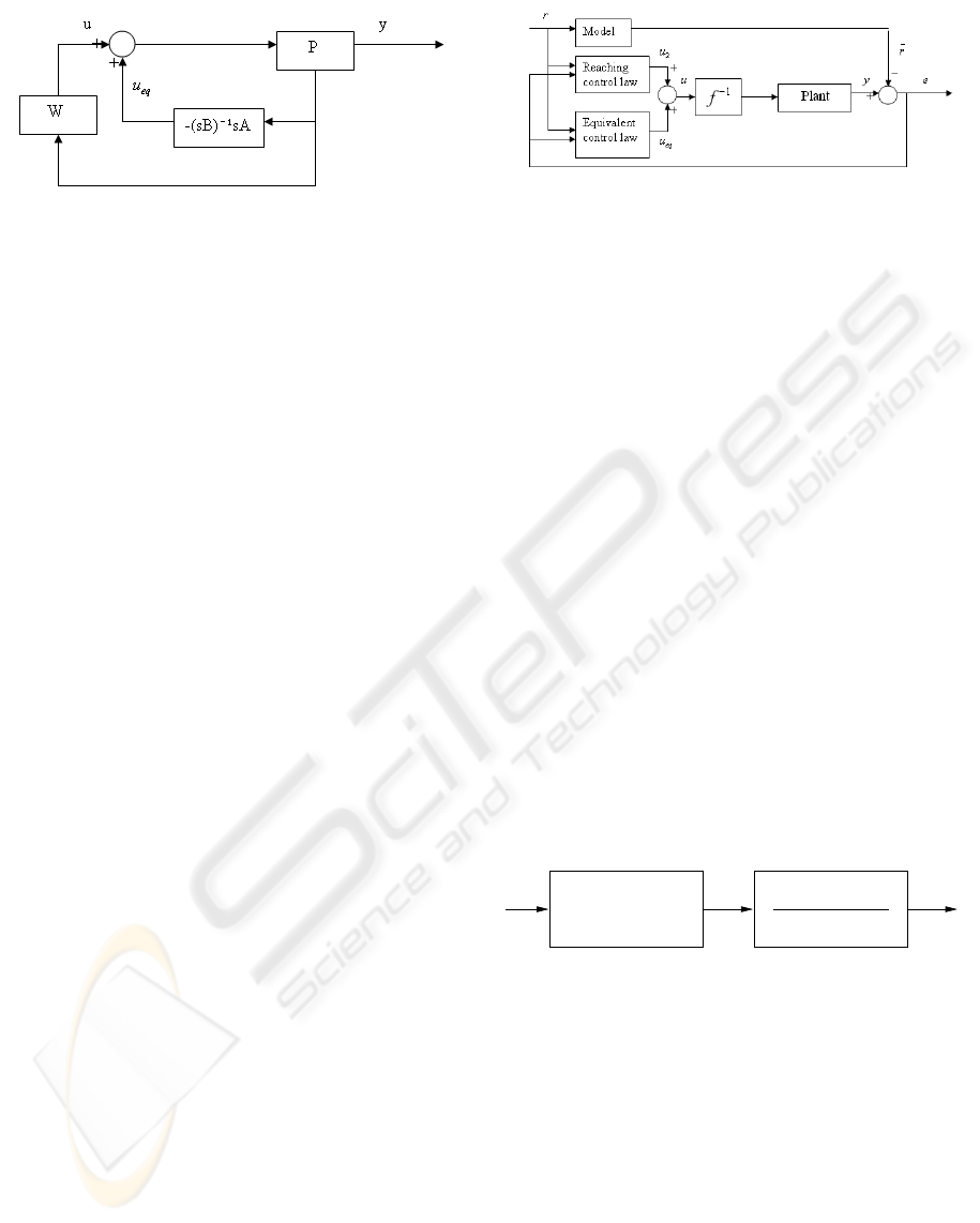
Figure 2: Structure of closed loop sliding mode control sys-
tem.
3.3 Sliding Mode Control for a
Hammerstein Model
In a Hammerstein model, the nonlinearity has been
separated from the linear block already. The nonlinear
mapping f is a smooth polynomial with respect to its
input, hence it is invertible. Thus in the controller
design stage, the nonlinearity can be ignored and the
controller is only designed based on the linear block
and afterwards, the control signal is filtered through
an inverse of the nonlinearity before being sent to the
plant. This may not be necessary if the nonlinearity is
taken into account in the Lyapunov function used for
determination of the reaching control.
As far as the description of the linear block is con-
cerned, a non-minimal state space model is employed
(refer to (Xi and Hesketh) for details of derivation of
non-minimal state space models). The motivation for
this is that in a non-minimal state space model, the er-
ror signal sequence is contained in state vector (the er-
ror signal being the difference between the plant out-
put and the desired trajectory). Sliding mode control
results in a regulator, where the state variables will
be constrained to move along the sliding surface and
eventually reach and stay at zero. Thus the error sig-
nal will be regulated to approach zero and stay there
if the sliding mode control is based on a non-minimal
state space model. This is the aim of tracking con-
trol. Figure 3. shows the structure of such a control
system.
In the figure, r represents the set point and e is
the difference between filtered set point and the out-
put of plant (Xi and Hesketh). For our example, the
“filter” is selected simply as q
−1
. Here both equiva-
lent and reaching controller are related to the tracking
error and the set point. The control action force the
states to reach the sliding manifold and move along it.
This action continues until the plant output is equal to
the filtered set point, which is equivalent to the error
signal being zero. Then the states will be kept at the
Figure 3: Structure of sliding mode control system based on
Hammerstein model.
origin and the system achieves steady state.
4 EXAMPLE AND SIMULATION
RESULTS
4.1 Identification of Ball and Beam
Deriving an approximate model of the ball and beam
system involves determining the transfer function be-
tween the input signal (the shaft angle of the mo-
tor) and the output signal (the position of the ball).
In an identification experiment, a pseudo-random se-
quence is applied to the input signal, and both in-
put and output signals are sampled (For the ball and
beam the sampling interval selected was 1 second).
Here Captain Toolbox which is written for Matlab is
used to realize the identification ((Young et al., 2001),
http://www.es.lancs.ac.uk/cres/captain/). The result
of the Hammerstein model identification is:
y(t) = 0.962y(t −1)+0.396u(t − 1) − 0.036u
2
(t − 1)
u x
y
0.396u(t)−0.036u (t)
2
q
−1
1−0.962q
−1
Figure 4: Identification result of Hammerstein model.
The resultant non-minimal state space model of
the linear block is:
z(t) = Az(t − 1) + B∆x+ Q∆r(t) (28)
y(t) = Cz(t) (29)
where
A =
1.962 −0.962 −1 0.962
1 0 0 0
0 0 0 0
0 0 1 0
, B =
1
0
0
0
,
C =
1 0 0 0
, Q =
0
0
1
0
, z(t) =
e
eq
−1
∆r
∆rq
−1
.
SLIDING MODE CONTROL FOR HAMMERSTEIN MODEL BASED ON MPC
235
Suitable differencing is undertaken to introduce
∆ = 1 − q
−1
. Note the way in which the setpoint
is introduced within the state vector. This results in
feedforward action, achieved with the sliding mode
control.
4.2 Controller Design and Simulation
This system is typically unobservable. Performing of
observable/unobservable decomposition prevents sin-
gularity occurrence later. The system model becomes:
−
z(t) =
−
A
−
z(t − 1) + B∆
−
x(t − 1) + Q
ob
∆r(t)(30)
−
y(t) =
−
C
−
z(t) (31)
where the transformation matrix is T and
−
A =
0 0.5698 0.4188 0.7071
0 0.3374 0.2480 −0.4188
0 −0.4591 −0.3374 0.5698
0 0 −1.6885 1.962
,
−
B =
0
0
0
1
,
−
C =
0 0 0 1
.
Extracting the observable part we have:
z
ob
(t) = A
ob
z
ob
(t −1) + B
ob
∆u
ob
(t −1) (32)
y
ob
(t) = C
ob
z
ob
(t) (33)
where
A
ob
=
0.3374 0.2480 −0.4188
−0.4591 −0.3374 0.5698
0 −1.6885 1.962
, B
ob
=
0
0
1
.
In this case, the requirement of equation (5) has al-
ready been satisfied so that no further transformation
P is needed. Then
A
ob11
=
0.3374 0.248
−0.4591 −0.3374
, A
ob12
=
−0.4188
0.5698
,
A
ob21
=
0 −1.6885
, A
ob22
= [1.962]
The result of optimization is
k
1
k
2
.
Note that an inversion of the observ-
able/unobservable decomposition is to be performed
to recover the state vector z
ob
(t) = Tz(t) after sliding
surface design,
σ(z
ob
(t)) =
k
1
k
2
1
z
ob
(t) (34a)
σ(z(t)) =
k
1
k
2
1
Tz(t) = sz(t).(34b)
In this case, u
2
(t) is chosen to be −αsgn(σ(x(t))).
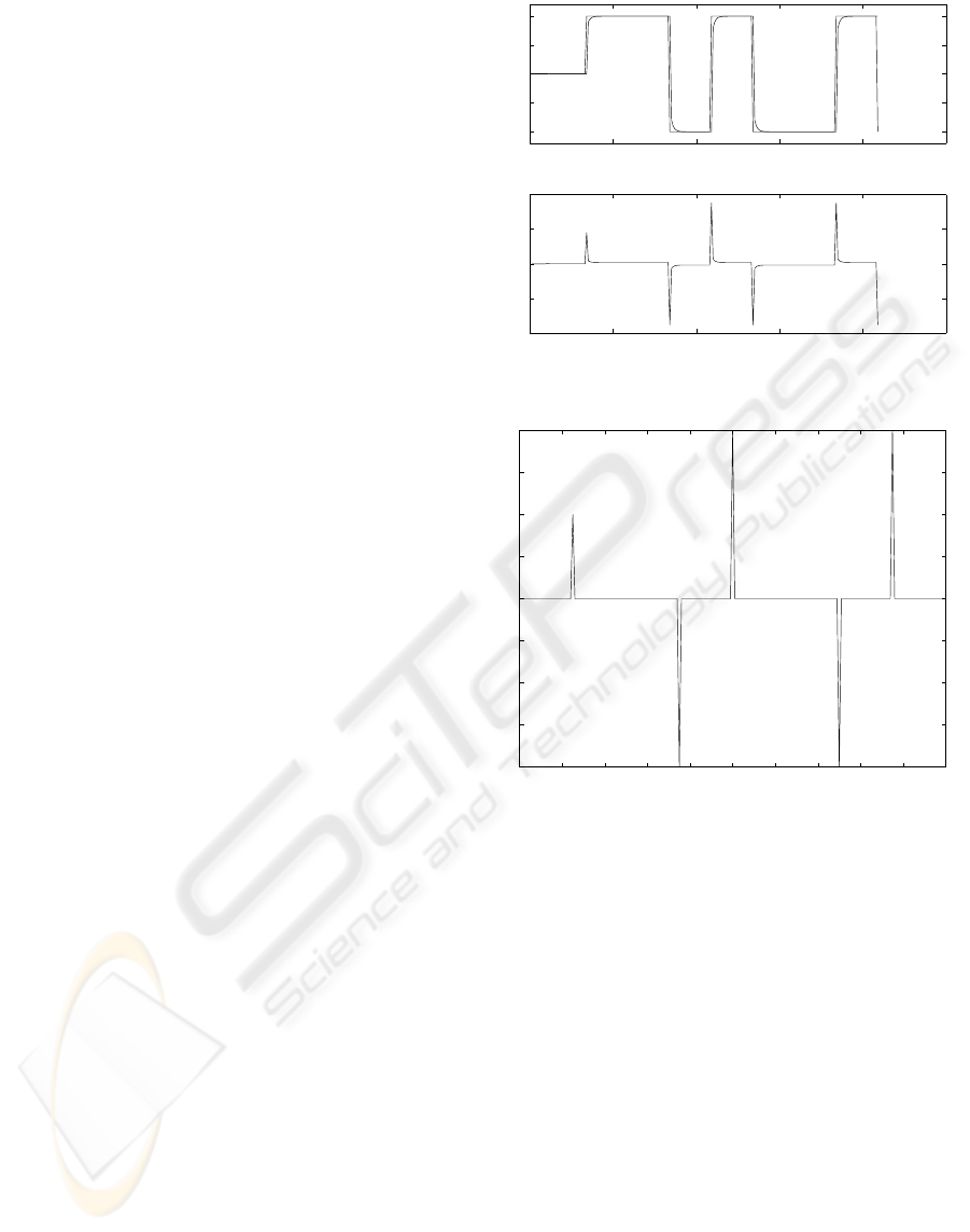
Figure 5. shows the performance of the above sliding
0 50 100 150 200 250
−1
−0.5
0
0.5
1
y and rbar
0 50 100 150 200 250
−2
−1
0
1
2
u
Figure 5: Performance with a linear model.
0 20 40 60 80 100 120 140 160 180 200
−0.2
−0.15
−0.1
−0.05
0
0.05
0.1
0.15
0.2
Figure 6: σ(t) defined in equation (13).
mode design. The figure shows simulation results, but
on-line control is similar.
Figure 6. shows the values of σ(t) And Figure 7.
shows the state trajectory:
It is shown that the system follows the ideal trajec-
tory. The switching law works while sliding condition
is not met. Equivalent control regulates the state to
move along the sliding surface until the equilibrium
point is achieved.
5 CONCLUSION
In this paper, discrete sliding mode control is applied
to a Hammerstein model which results from nonlinear
system identification. The nonlinearity is separated
during the sliding surface design, so that the switch-
ing surface is actually a linear one. The surface is
derived by an MPC approach. The nonlinearity is re-
ICINCO 2007 - International Conference on Informatics in Control, Automation and Robotics
236
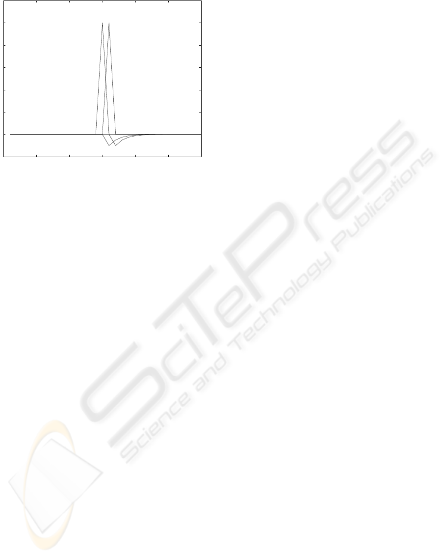
0 5 10 15 20 25 30
−0.2
0
0.2
0.4
0.6
0.8
1
1.2
Figure 7: State variables.
considered in design of the reaching control. The ball
and beam system is used as an example and simula-
tion results show satisfying performance.
REFERENCES
Bitmead, R. R., Gevers, M., and Wertz, V., 1990,
Adaptive
Optimal Control: The Thinking man’ s GPC (Prentice
Hall)
.
Clarke, D. W., Mohtadi, C., and Tuffs, P. S., 1987,
General-
ized Predictive Control– Part I. The Basic Algorithm
,
Automatica, 23, 137- 148;
Clarke, D. W., Mohtadi, C., and Tuffs, P. S., 1987,
General-
ized Predictive Control–Part II. Extensions and Inter-
pretations
, Automatica, 23, 149-160
C. James Taylor, Arun Chotai and Peter C. Young, 2000,
State space control system design based on non-
minimal state-variable feedback: further generaliza-
tion and unification results
, International Journal of
Control, 2000, Vol. 73, No. 14, 1329- 1345
Raymond, A DeCarlo, Stanislaw H. Zak, Gregory
P.Matthews,
Variable Structure Control of Nonlinear
Multivariable Systems: A Tutorial
, Proceedings of
The IEEE, Vol. 76, No. 3, March 1988
S. K. Spurgeon,
Temperature Control of Industrial Process
using a Variable Structure Design Philosophy
, Trans
Inst MC Vol. 14, No. 5, 1992
Stefen Hui, Stanislaw H. Zak,
On discrete-time variable
structure sliding mode control
, Systems & Control
Letters 38 (1999) 283-288
Weibong Gao, Yufu Wang, Abdollah Homaifa,
Discrete-
Time Variable Structure Control Systems
, IEEE
Transactions on Industrial Electronics, Vol. 42, No.2,
April 1995
Jozef Voros,
System Identification of Discontinuous Ham-
merstein Systems,
Automatica Vol.33.No.6. pp. 1141-
1146, 1997
F. Giri, F. Z. Chaoui, Y. Rochdi,
Parameter identification of
a class of Hammerstein plants
, Automatica, 37 (2001)
749-756
Xinghuo Yu and Guanrong Chen,
Discretization Behav-
iors of Equivalent Control Based Sliding-Mode Con-
trol Systems
, IEEE Transaction On Automatic Con-
trol, Vol. 48, No. 9, September 2003
Xinghuo Yu, Shuanghe Yu,
Discrete Sliding Mode Control
Design With Invariant Sliding Sectors
, Transaction of
the ASME, Vol. 122, Page776-782, December 2000.
Zhiyu Xi, Tim Hesketh,
MPC With a NMSS Model
, The
Sixth International Conference on Control and Au-
tomation.
Peter C. Young, Paul McKenna, John Brunn,
Identification
of Nonlinear Stochastic Systems by State Dependent
Parameter Estimation
, International Journal of Con-
trol, 2001, Vol. 74, No. 18, 1837-1857
C. L. Hwang and J. C. Hsu,
Nonlinear control design for a
Hammerstein model system
, IEE Procedings, Control
Theory and Applications, Vol 142, Issue 4, p.p 277-
285
Zi Ma, Arthur Jutan, Vladimir B. Bajic,
Nonlinear self-
tuning controller for Hammerstein plants with appli-
cation to a pressure tank
. Int. J. Comput. Syst. Signal,
1(2), 221-230, 2000
SLIDING MODE CONTROL FOR HAMMERSTEIN MODEL BASED ON MPC
237
