DETECTION OF THE NEED FOR A MODEL UPDATE IN STEEL

MANUFACTURING

Heli Koskim

aki (n

ee Junno), Ilmari Juutilainen, Perttu Laurinen and Juha R

oning

Intelligent Systems Group, University of Oulu, PO BOX 4500,90014 University of Oulu, Finland

Keywords:

Adaptive model update, similar past cases, error in neighborhood, process data.

Abstract:

When new data are obtained or simply when time goes by, the prediction accuracy of models in use may

decrease. However, the question is when prediction accuracy has dropped to a level where the model can

be considered out of date and in need of updating. This article describes a method that was developed for

detecting the need for a model update. The method is applied in the steel industry, and the model whose need

of updating is under study is a regression model developed to model the yield strength of steel plates. It is used

to plan process settings in steel plate product manufacturing. To decide on the need for updating, information

from similar past cases was utilized by introducing a limit called an exception limit. The limit was used to

indicate when a new observation was from an area of the model input space where the prediction errors of the

model have been too high. Moreover, an additional limit was formed to indicate when too many exceedings of

the exception limit have occurred within a certain time scale. These two limits were then used to decide when

to update the model.

1 INTRODUCTION

At the Ruukki’s steel works in Raahe, Finland, liq-

uid steel is cast into steel slabs that are then rolled

into steel plates. Many different variables and mech-

anisms affect the mechanical properties of the ﬁnal

steel plates. The desired speciﬁcations of the me-

chanical properties of the plates vary, and to fulﬁll

the speciﬁcations, different treatments are required.

Some of these treatments are complicated and ex-

pensive, so it is possible to optimize the process by

predicting the mechanical properties beforehand on

the basis of planned production settings (Khattree and

Rao, 2003).

Regression models have been developed for

Ruukki to help development engineers control me-

chanical properties such as yield strength, tensile

strength, and elongation of the metal plates (Juuti-

lainen and R

oning, 2006). However, acquirement of

new data and the passing of time decrease the reliabil-

ity of the models, which can bring economical losses

to the plant. For example, when mechanical proper-

ties required by the customer are not satisﬁed in qual-

iﬁcation tests, the testing lot in question need to be re-

produced. If also retesting gives unsatisfactory result

the whole order has to be produced again. Because of

the volumes produced in a steel mill, this can cause

huge losses. Thus, updating of the models emerges as

an important step in improving modelling in the long

run. This study concerns the need to update the re-

gression model developed to model the yield strength

of steel plates.

In practice, because the model is used in ad-

vance to plan process settings and since the employ-

ees know well how to produce common steel plate

products, modelling of rare and new events becomes

the most important aspect. However, to make new

or rarely manufactured products, a reliable model is

needed. Thus, when comparing the improvement in

the model’s performance, rare events are emphasized.

In this study, model adaptation is approached by

searching for the exact time when the performance

of the model has decreased too much. In practice,

model adaptation means retraining the model at opti-

mally selected intervals. However, because the sys-

tem has to adapt quickly to a new situation in order to

Koskimäki (née Junno) H., Juutilainen I., Laurinen P. and Röning J. (2007).

DETECTION OF THE NEED FOR A MODEL UPDATE IN STEEL MANUFACTURING.

In Proceedings of the Fourth International Conference on Informatics in Control, Automation and Robotics, pages 55-59

DOI: 10.5220/0001639500550059

 SciTePress

avoid losses to the plant, periodic retraining, used in

many methods ((Haykin, 1999), (Yang et al., 2004)),

is not considered the best approach. Moreover, there

are also disadvantages if retraining is done unneces-

sarily. For example, extra work is needed to take a

new model into use in the actual application environ-

ment. In the worst case, this can result in coding er-

rors that affect the actual accuracy of the model.

Some other studies, for example (Gabrys et al.,

2005), have considered model adaptation as the

model’s ability to learn behavior in areas from which

information has not been acquired. In this study,

adaptation of the model is considered to be the ability

to react to time-dependent changes in the modelled

causality. In spite of extensive literature searches,

studies that would be comparable with the approach

used in this article were not found. Thus, it can be

assumed that the approach is new, at least in an actual

industrial application.

2 DATA SET AND REGRESSION

MODEL

The data for this study were collected from the

Ruukki’s steel works production database between

July 2001 and April 2006. The whole data set con-

sisted of approximately 250,000 observations. In-

formation was gathered from element concentrations

of actual ladle analyses, normalization indicators,

rolling variables, steel plate thicknesses, and other

process-related variables (Juutilainen et al., 2003).

The observations were gathered during actual product

manufacturing. The volumes of the products varied,

but if there were more than 500 observations from one

product, the product was considered a common prod-

uct. Products with less than 50 observations were cat-

egorized as rare products.

The response variable used in the regression mod-

elling was the Box-Cox-transformed yield strength of

the steel plates. The Box-Cox transformation was se-

lected to produce a Gaussian-distributed error term.

The studied regression model was a link-linear model

= µ

+ ε

, where µ

= f(x

β) and ε

are indepen-

dently distributed Gaussian errors. The length of the

parameter vector β was 130. In addition to 30 orig-

inal input variables, the input vector x

included 100

carefully chosen non-linear transformations of origi-

nal input variables; for example, many of these trans-

formations were products of two or three original in-

puts. The results are presented in the original (non-

transformed) scale of the response variable.

3 NEIGHBORHOOD AND APEN

In this study the need for a model update was

approached using information from previous cases,

namely the average prediction errors of similar past

cases. Thus, for every new observation, a neighbor-

hood containing similar past cases was formed and an

average prediction error inside the neighborhood was

calculated.

The neighborhoods were deﬁned using a Euclid-

ian distance measure and the distance calculation was

done only for previous observations to resemble the

actual operating environment. The input variables

were weighted using gradient-based scaling, so the

weighting was relative to the importance of the vari-

ables in regression model (Juutilainen and R

oning,

ress). A numerical value of 3.5 was considered for

the maximum distance inside which the neighboring

observations were selected. The value was selected

using prior knowledge of the input variable values.

Thus, a signiﬁcant difference in certain variable val-

ues with the deﬁned weighting resulted in Euclidean

distances of over 3.5. In addition to this, the maxi-

mum count of the selected neighbors was restricted to

500.

After the neighborhood for a new observation was

deﬁned, the average prediction error of the neigh-

borhood (= APEN) was calculated as the distance-

weighted mean of the prediction errors of observa-

tions belonging to the neighborhood:

APEN =

∑

i=1

[(1−

max(d)

) ·

]

∑

i=1

(1−

max(d)

)

, (1)

where

n = number of observations in a neighbor-

hood,

ε(i) = the prediction error of ith observation

of the neighborhood,

= the Euclidian distance from the new

observation to ith observation of the

neighborhood,

max(d) = the maximum allowed Euclidian dis-

tance between the new observation

and the previous observations in the

neighborhood (= 3.5).

ICINCO 2007 - International Conference on Informatics in Control, Automation and Robotics

4 STUDY

The method used to observe the need for a model up-

date was to determine when the model’s average pre-

diction error in the neighborhood of a new observa-

tion (APEN) differed from zero too much compared

with the amount of similar past cases. When there are

plenty of accurately predicted similar past cases, the

APEN is always near zero. When the amount of sim-

ilar past cases decreases, the sensitivity of the APEN

(in relation to measurement variation) increases, also

in situations when the actual model would be accu-

rate. In other words, the relationship between the

sensitivity of the APEN and the number of neighbors

is negatively correlated. The actual updating is also

time-dependent, which means the model is updated

when too many observations have an APEN value that

differs signiﬁcantly from zero within a certain time

interval.

A limit, called the exception limit, was introduced

to detect the need to update the model. The limit de-

ﬁnes how high the absolute value of the average pre-

diction error of a neighborhood (= |APEN|) has to

be in relation to the size of the neighborhood before

it can be considered an exception. This design was

introduced to avoid possible sensitivity issues of the

APEN. In practice, if the size of the neighborhood

was 500 (the area is well known), prediction errors

higher than 8 were deﬁned as exceptions, while with

a neighborhood whose size was 5, the error had to be

over 50. The values of the prediction errors used were

decided by relating them to the average predicted de-

viation,

(≈ 14.4). The predicted deviations were

acquired by using a regression model (Juutilainen and

oning, 2006). The limit is shown in Figure 1.

0 50 100 150 200 250 300 350 400 450 500

Size of neighborhood

Average estimation error

Figure 1: Exception limit.

A second limit, the update limit, was deﬁned as

being exceeded if 10 percent of the average predic-

tion errors of the neighborhoods within a certain time

interval exceeded the exception limit. The chosen in-

terval was 1000 observations, which represents mea-

surements from approximately one week of produc-

tion. Thus, the model was retrained every time 100 of

the preceding 1000 observations exceeded the excep-

tion limit.

The study was started by training the parameters

of the regression model using the ﬁrst 50,000 observa-

tions (approximately one year). After that the trained

model was used to give the APENs of new observa-

tions. The point where the update limit was exceeded

the ﬁrst time was located and the parameters of the

model were updated using all the data acquired by

then. The study was carried on by studying the relia-

bility of the model after each update and repeating the

steps iteratively until the whole data set was passed.

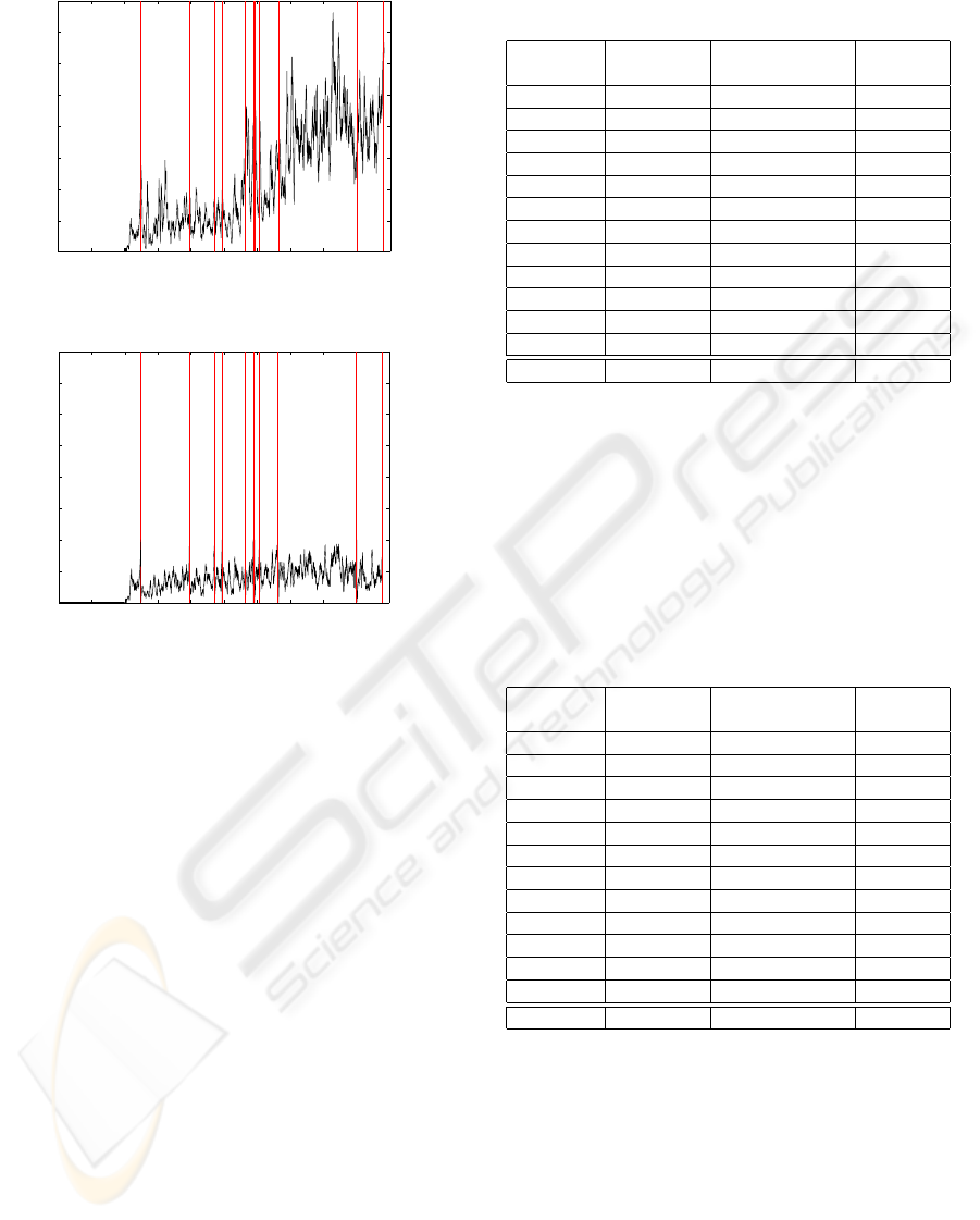
5 RESULTS

First the reliability of the model with and without up-

dating was studied. Figure 2 shows the average pre-

diction errors of the respective neighborhoods. Fig-

ure 2(a) shows the model’s performance without up-

dating. The straight line in the beginning represents

the training data and the rest of the curve shows the

proportional share of the exceedings of the exception

limit, in other words, the percentage of APENs that

exceeded the exception limit. For example, it can be

seen that at the end of the curve the APEN of every

fourth new observation per week has exceeded the ex-

ception limit. The vertical lines mark the points of

iteration where the update limit has been exceeded.

On the other hand, Figure 2(b) presents the reliability

of the model when the parameters are re-estimated at

times indicated by the vertical lines. The curve repre-

sents the error rate of the re-trained model.

The positive effect of the updates on the average

prediction errors of the neighborhoods can be clearly

seen from Figure 2. Therefore, it is evident that the

model’s performance increases when the developed

updating strategy is applied.

Although the reliability information of the model

is very useful, the effect of the update on the actual

prediction error was considered more important. Two

different goodness criteria were used to compare the

actual prediction errors of the updated models. Both

criteria emphasize rare events, because that is the case

when the model is needed the most. Both of them

show the weighted average of the absolute prediction

errors, with different weighting schemes.

In the ﬁrst goodness criterion the idea is to em-

phasize all the products by approximately an equal

amount. This means that in the calculation of the

average prediction error, the weights of observations

DETECTION OF THE NEED FOR A MODEL UPDATE IN STEEL MANUFACTURING

0 0.25 0.5 0.75 1 1.25 1.5 1.75 2 2.25 2.5

x 10

0.05

0.1

0.15

0.2

0.25

0.3

0.35

0.4

The observation number

The proportional share of deviations (window size 1000)

(a) Without update.

0 0.25 0.5 0.75 1 1.25 1.5 1.75 2 2.25 2.52.5

x 10

0.05

0.1

0.15

0.2

0.25

0.3

0.35

0.4

The observation number

The proportional share of deviations (window size 1000)

(b) With update.

Figure 2: Reliability of the model.

belonging to products having more than 50 observa-

tions are decreased. The results of the goodness cri-

terion are shown in Table 1. The step size indicates

the length of the iteration step (comparable with the

space between the vertical lines in Figure 2). The re-

sults are averages of the absolute prediction errors of

the observations between each iteration step. Thus,

the size of the data set used to calculate the average

is the same as the step size. In addition to this, to

compare the results, the prediction error averages are

presented in three different cases: predicted with a

newly updated model, with a model updated in the

previous iteration step, and with a model that was not

updated at all. The results show that, although the dif-

ferences between the new model and the model from

the previous iteration step are not big, the update im-

proves the prediction in each of the steps. The beneﬁt

of the model update is obvious when the results of the

updated model and the model without an update are

compared.

The second goodness criterion was formed to take

only rare events into account. Thus, only the cases

Table 1: Means of absolute prediction errors with the ﬁrst

goodness criterion.

Step size With new With previous Without

model model update

12228 - - -

36812 11.59 11.74 11.74

18826 10.47 11.00 10.69

5623 10.93 11.08 11.25

17636 12.48 12.57 12.97

6165 11.48 12.38 13.31

699 29.92 30.20 41.00

3765 11.79 12.21 13.96

14317 12.35 12.42 13.53

59432 12.22 12.39 12.87

19455 12.72 13.46 14.81

507 11.46 11.68 15.22

mean 12.07 12.32 12.79

where the neighborhood size is smaller than 50 are

considered. The absolute prediction errors of these

rare observations affect the average equal amount.

The update proves its functionality in this scheme,

also. The prediction errors are notably smaller when

the model is updated (see Table 2).

Table 2: Means of absolute prediction errors with the sec-

ond goodness criterion.

Step size With new With previous Without

model model update

12228 - - -

36812 14.41 14.63 14.63

18826 13.14 14.12 13.99

5623 12.94 13.11 13.10

17636 16.48 16.60 18.22

6165 12.60 13.90 14.71

699 84.86 85.86 115.44

3765 13.88 17.08 21.28

14317 16.23 16.21 22.09

59432 15.42 15.54 17.90

19455 26.42 27.88 43.87

507 15.99 15.18 16.04

mean 15.67 16.04 18.10

With this data set, determination of the need for

a model update and the actual update process proved

their efﬁciency. The number of iteration steps seems

to be quite large, but like in Figure 2, the iteration

steps get longer when more data is used to train the

model. Thus, the amount of updates decreases as time

goes on. However, the developed approach can also

adapt to changes rapidly, when needed, as when new

products are introduced or the production method of

an existing product is changed. Finally, the beneﬁts of

this more intelligent updating procedure are obvious

ICINCO 2007 - International Conference on Informatics in Control, Automation and Robotics

in comparison with a dummy periodic update proce-

dure (when the model is updated at one-year intervals,

for example, the prediction error means of the whole

data sets are 12.24 using criterion 1 and 16.34 using

criterion 2, notably worse than the results achieved

with our method, 12.07 and 15.67). The periodic pro-

cedure could not react to changes quickly or accu-

rately enough, and in some cases it would react un-

necessarily.

6 CONCLUSIONS

This paper described the development of a method for

detecting the need for a model update in the steel in-

dustry. The prediction accuracy of regression mod-

els may decrease in the long run, and a model update

at periodic intervals may not react to changes rapidly

and accurately enough. Thus, there was a need for a

reliable method for determining suitable times to up-

date the model. Two limits were used to detect these

update times, and the results appear promising. In

addition, it is possible to rework the actual values of

the limits to optimize the updating steps and improve

the results before implementing the method in an ac-

tual application environment. Although the procedure

was tested using a single data set, the extensiveness of

the data set clearly proves the usability of the proce-

dure. Nevertheless, the procedure will be validated

when it is adapted also to regression models devel-

oped to model the tensile strength and elongation of

metal plates.

In this study the model update was performed by

using all the previously gathered data to deﬁne the re-

gression model parameters. However, in the future the

amount of data will increase, making it hard to use all

the gathered data in an update. Thus, new methods for

intelligent data selection are needed to form suitable

training data. In addition, the model update could be

developed into a direction where the input variables

of the regression model can also be changed during

the update.

REFERENCES

Gabrys, B., Leivisk

a, K., and Strackeljan, J. (2005). Do

Smart Adaptive Systems Exist, A Best-Practice for

Selection and Combination of Intelligent Methods.

Springer-Verlag, Berlin, Heidelberg.

Haykin, S. (1999). Neural Networks, A Comprehensive

Foundation. Prentice Hall, Upper Saddle River, New

Jersey.

Juutilainen, I. and R

oning, J. (2006). Planning of strength

margins using joint modelling of mean and dispersion.

Materials and Manufacturing Processes, 21:367–373.

Juutilainen, I. and R

oning, J. (2007, in press). A method for

measuring distance from a training data set. Commu-

nications in Statistics.

Juutilainen, I., R

oning, J., and Myllykoski, L. (2003). Mod-

elling the strength of steel plates using regression

analysis and neural networks. Proceedings of Interna-

tional Conference on Computational Intelligence for

Modelling, Control and Automation, pages 681–691.

Khattree, R. and Rao, C., editors (2003). Statistics in indus-

try - Handbook of statistcs 22. Elsevier.

Yang, M., Zhang, H., Fu, J., and Yan, F. (2004). A

framework for adaptive anomaly detection based on

support vector data description. Lecture Notes in

Computer Science, Network and Parallel Computing,

pages 443–450.

DETECTION OF THE NEED FOR A MODEL UPDATE IN STEEL MANUFACTURING