
HIERARCHICAL SPLINE PATH PLANNING METHOD FOR
COMPLEX ENVIRONMENTS
Martin Saska, Martin Hess and Klaus Schilling
University of Wuerzburg, Germany
Informatics VII, Robotics and Telematics
Am Hubland, Wuerzburg, Germany, 97074
Keywords:
Path planning, Mobile robots, PSO, Spline path, Hierarchical approach.
Abstract:
Path planning and obstacle avoidance algorithms are requested for robots working in more and more compli-
cated environments. Standard methods usually reduce these tasks to the search of a path composed from lines
and circles or the planning is executed only with respect to a local neighborhood of the robot. Sophisticated
techniques allow to find more natural trajectories for mobile robots, but applications are often limited to the
offline case.
The novel hierarchical method presented in this paper is able to find a long path in a huge environment with
several thousand obstacles in real time. The solution, consisting of multiple cubic splines, is optimized by
Particle Swarm Optimization with respect to execution time and safeness. The generated spline paths result in
smooth trajectories which can be followed effectively by nonholonomic robots.
The developed algorithm was intensively tested in various simulations and statistical results were used to
determine crucial parameters. Qualities of the method were verified by comparing the method with a simple
PSO path planning approach.
1 INTRODUCTION
Expanding mobile robotics to complicated envi-
ronments increases the requirements on the con-
trol system of the robot. The desired task has
to be executed by the robot as fast as possible in
these scenarios. Standard path planning approaches
very often just provide simple piecewise constant
routes (Latombe, 1996),(Kunigahalli and Russell,
1994),(Franklin et al., 1985) or only local optimal so-
lutions (Borenstein and Koren, 1991),(Khatib, 1986).
Few methods that give continues and smooth solu-
tion (Azariadis and Aspragathos, 2005), (Nearchou,
1998), due to long computational time in order of
minutes, cannot be used in real time applications.
All path planning methods try to find a path from an
actual position S of the controlled robot to a desired
goal position G, with regard to position and shape of
known obstacles O. While these parameters stand as
the inputs of the algorithm, the output can be either an
optimal path from S to G or just a direction from the
actual position respecting locally optimal trajectory.
The key issue of the path planning for mobile robots
is how to define the best trajectory. A common an-
swer to this is that the optimal path should be similar
to a path designed by a human operator. This vague
definition can be expressed by a penalty function that
is minimized during the planning. The simplest ver-
sion of the function consists of two parts. While the
first one evaluates a length of the path (or time needed
to goal fulfilment), the second part ensures safety of
the path (i.e. sufficient distance to obstacles). So find-
ing an acceptable compromise between these require-
ments is the core problem of the path planning itself.
The novel approach presented in this paper offers
a solution to the above mentioned problems. The
output of the algorithm is a path, which consists of
smoothly connected cubic splines. Spline paths are
naturally executable by the robot and optimization
of the speed profile can be easily done by modifica-
tions of the radius of the curvature. Global informa-
tion about the workspace is subsumed, because the
whole space of spline trajectories from S to G will
be searched through during the optimization process.
Therefore big clusters of obstacles as well as huge
obstacles in the environment can be avoided imme-
diately. This enables us to locate the final solution in
the areas with lower density of obstacles at the begin-
ning of the mission. Such a path may seem longer,
due to necessary deviations from the ”bee-line”, but
116
Saska M., Hess M. and Schilling K. (2007).
HIERARCHICAL SPLINE PATH PLANNING METHOD FOR COMPLEX ENVIRONMENTS.
In Proceedings of the Fourth International Conference on Informatics in Control, Automation and Robotics, pages 116-123
DOI: 10.5220/0001640001160123
Copyright
c
SciTePress
the final movement time can be shorter, because diffi-
cult maneuvers in the obstacle clusters are eliminated.
Particle Swarm Optimization (PSO) (Eberhart and
Kennedy, 1995) was used for prospecting the optimal
solution hereunder due to its relatively fast conver-
gence, its global search character and its ability to
avoid local minima. In this paper is supposed real
time path planning and therefore the solution must
be given in a split second. The complexity of PSO
strongly depends on the dimension of the search space
and on the needed swarm size. The number of iter-
ations increase more than exponentially with the di-
mension. Accordingly a minimal length of the parti-
cle is required, but in complex environments a short
string of cubic splines is not sufficient and collision
free path in such limited space often does not exist.
In the proposed algorithm, that is based on a hi-
erarchical approach, the PSO process is used several
times. Each optimization proceeds in a subspace with
a small dimension, but the total size of the final so-
lution can be unlimited. The path obtained by this
method is only suboptimal, but the reduction of the
computational time is incomparable bigger. In addi-
tion the algorithm can be started without prior knowl-
edge about the complexity of the environment, be-
cause the dimension of the search space is specified
during the planning process. The dimension even may
not be uniform in the whole workspace, but it is au-
tomatically adapted according to the number of col-
lisions along the path, that is found by the hierarchi-
cally plunging.
The paper is organized as followed: A novel
method reflecting special requirements for the mobile
robots in a complex environment is presented in sec-
tion 2. Section 2.1 provides information about the
universal PSO approach. In section 2.2 adaptations
of the PSO to our specific problem are described. Af-
ter this experimental results are presented in section
3 followed by concluding words and plans for future
work in section 4.
2 PATH PLANNING
The path planning approach presented in this pa-
per is based on a searching through a space of
states P . Each state P
i
is represented by a vector
P
i
= (P
i,x
, P
i,y
, P
′
i,x
, P
′
i,y
), that denotes position and
heading of the robot in the workspace. The final path
of the robot is set by a transition P
i
T
i
→ P
i+1
between
each pair of neighboring states. T
i
can be defined
uniquely, if T ≡ C
1
, where C
1
is the set of cubic
splines with smooth first derivation (closely described
in 2.2).
The system of all solutions Π is a vector
Π = < S, G, p, t, f(t) >, where S, G ∈ P are start
and goal states of the robot and p ⊂ P is a sequence
of the states between S and G. t ⊂ T is a string of
the splines connecting S and G and f(t) is the fitness
function denoting the quality of the found path. The
solution π ∈ Π with minimum value of f (t) should
conform with the best path.
The crucial problem is to find π with minimum or
nearly minimum value of the fitness function in the
usually vast set Π. The complexity of the task grows
with the size of vector p. Solutions with a small
dimension of p can be found faster, but a collision
free path may not exist in such limited space, if the
workspace of the robot is too complicated.
Higher-level
planning
PSOmodule
Collision
detection
Control
module
MAP
Path
planning
Start,Goal
Control
points
Start
Goal
Controlpoints
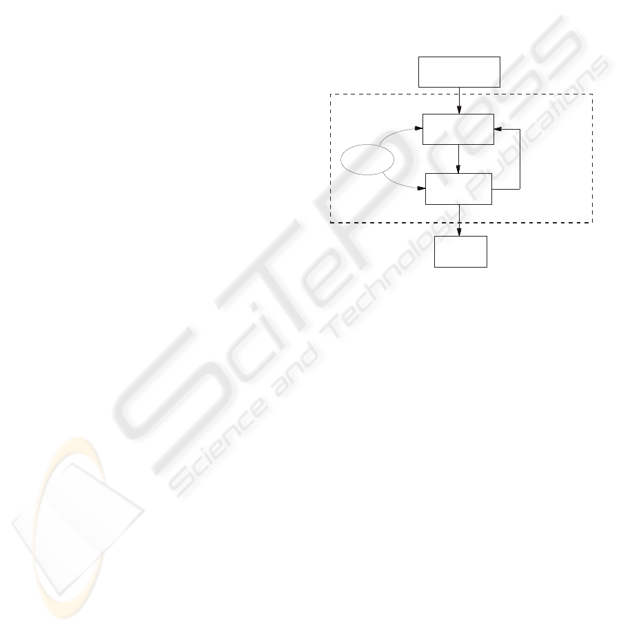
Figure 1: Schema of the presented hierarchical method.
In the hierarchical approach presented in this pa-
per the optimization task is decomposed to multiple
subtasks. The basic idea of the algorithm can be seen
in Fig. 1. The actual state of the robot and the de-
sired state generated by a higher planning module are
the inputs for the Particle Swarm Optimization (de-
scribed in 2.1). The path t which was found by PSO
is checked in the collision detection module and a
collision free solution is sent to the control module,
where the path is executed. If a collision is detected,
the string of splines t is divided and control points of
each spline are used as new input for the PSO module.
These points are put into the memory of the module
sequently. For other optimization processes always
the last added points are chosen. This ”LIFO” ap-
proach guarantees that the path close to the robot will
be found as soon as possible. The remaining path will
be found during the robot’s movement. Therefore the
time needed for the initial planning before the start of
the mission is reduced several times.
An example of the path decomposition is shown in
Fig. 2. Each vector p used in the optimization pro-
cesses contains only two states P
i
which correspond
to three splines in the string. In this simplified exam-
ple the hierarchical process is stopped always in the
third level, independently of the number of collisions.
HIERARCHICAL SPLINE PATH PLANNING METHOD FOR COMPLEX ENVIRONMENTS
117

The input states in each particle are printed with dark
background (e.g. S and G in the first level) whereas
the optimized states are represented by letters in white
rectangles (e.g. A and B in this level). The final path
in the lowest level consists of 27 splines and it is char-
acterized by 28 states of the robot. Such a path can be
found as an extreme of the nonlinear fitness function
in 104-dimensional space (26 optimized states mul-
tiplied by 4 numbers describing each state), which
is difficult (or impossible) in real time applications.
In the hierarchical approach the scanned space is 13
times reduced and the separate optimization subtask
can be done in tens of iterations. Furthermore only
three optimization processes (in the picture marked
by SABG, SCDA, SJKC) are necessary for the be-
ginning of the mission.
S
G
A
B
S GA B
G
S
A
B
B
A
A B
CD
E F
H I
J
C
C
D
D
E
E
F
F
H
H
I
I
K
L M
N
O
P
Q
R T
U
V
W
X
Y Z
a
b
Figure 2: Example of the path decomposition.
2.1 Particle Swarm Optimization
The PSO method was developed for finding a global
optimum of a nonlinear function (Kennedy and Eber-
hart, 1995),(Macas et al., 2006). This optimization
approach has been inspired by the social behavior of
birds and fish. Each solution consists of set of pa-
rameters and represents a point in a multidimensional
space. The solution is called ”particle” and the group
of particles (population) is called ”swarm”.
Two kinds of information are available to the parti-
cles. The first is their own experience, i.e. their best
state and it’s fitness value so far. The other informa-
tion is social knowledge, i.e. the particles know the
momentary best solution p
g
of the group found dur-
ing the evaluation process.
Each particle i is represented as a D-dimensional
position vector
−→
x
i
(q) and has a corresponding in-
stantaneous velocity vector
−→
v
i
(q). Furthermore, it
remembers its individual best value of fitness function
and position
−→
q
i
which has resulted in that value.
During each iteration t, the velocity update rule (1)
is applied on each particle in the swarm.
−→
v
i
(q) = w
−→
v
i
(q − 1) +
+ Φ
1
(
−→
p
i
−
−→
x
i
(q − 1)) +
+ Φ
2
(
−→
p
g
−
−→
x
i
(q − 1)) (1)
The parameter w is called inertia weight and during
all iterations decreases linearly from w
start
to w
end
.
The symbols Φ
1
and Φ
2
are computed according to
the equation
Φ
j
= ϕ
j
r
j1
0 0
0
.
.
.
0
0 0 r
jD
,
(2)
where j = 1, 2. The parameters ϕ
i
are constants
that weight the influence of the particles’ own experi-
ence and of the social knowledge. In our experiments,
the parameters were set to ϕ
1
= 2 and ϕ
2
= 2. The
r
jk
, where k = 1 . . . D are random numbers drawn
from a uniform distribution between 0 and 1.
The position of the particles is then computed ac-
cording to the update rule
−→
x
i
(q) =
−→
x
i
(q − 1) +
−→
v
i
(q). (3)
If any component of
−→
v
i
is less than −V
max
or
greater than +V
max
, the corresponding value is re-
placed by −V
max
or +V
max
, respectively, where
V
max
is the maximum velocity parameter.
Influencing V
max
in the simple PSO path planning
method (Saska et al., 2006b) illustrated a strong cor-
relation between the optimal value of the parameter
and the space’s size. This size is different for each
optimization process in the hierarchical tree, because
it is constrained by the position of the points S and
G. Therefore the value of V
max
is computed by the
equation
V
max
=
||S − G||
c
V
, (4)
where c
V
is a constant that has to be found experi-
mentally.
The update formulas (1) and (3) are applied during
each iteration and the values of p
i
and p
g
are updated
simultaneously. The algorithm is stopped if the maxi-
mum number of iterations is reached or any other pre-
defined stopping criteria is satisfied.
2.2 Particle Description and
Evaluation
The path planning for a mobile robot can be realized
by a search in the space of functions. We reduce this
space to a sub-space which only contains strings of
cubic splines. The mathematic notation of a cubic
spline (Ye and Qu, 1999) is
g(t) = At
3
− Bt
2
+ Ct + D, (5)
where t is within the interval < 0, 1 > and the
constants A, B, C, D are uniquely determined by
the boundary conditions g(0) = P
0
, g(1) = P
1
,
g
′
(0) = P
′
0
and g
′
(1) = P
1
:
ICINCO 2007 - International Conference on Informatics in Control, Automation and Robotics
118
A = 2P
0
− 2P
1
+ P
′
0
+ P
′
1
(6)
B = −3P
0
+ 3P
1
− 2P
′
0
− P
′
1
(7)
C = P
′
0
(8)
D = P
0
. (9)
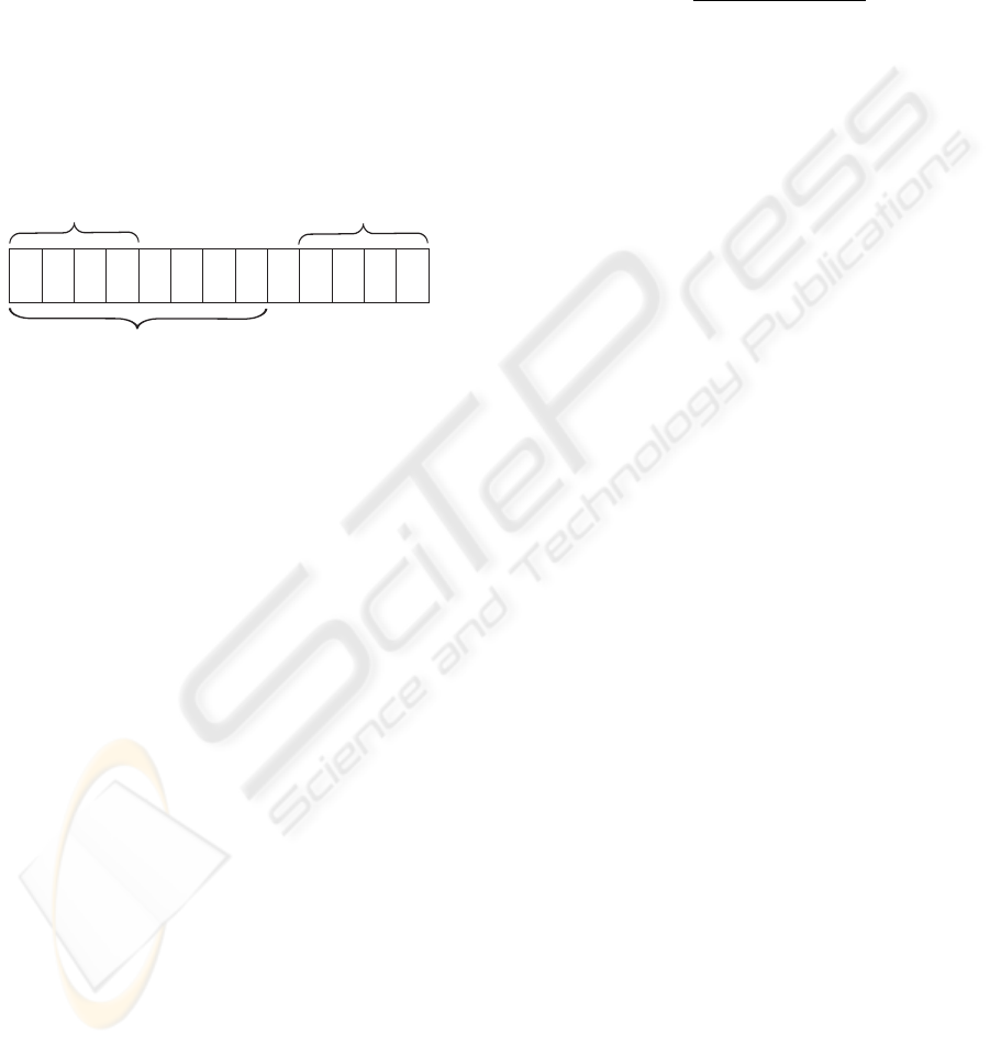
To guarantee continuity in the whole path, every
two neighboring splines in the string must share one
of their terminal states and therefore the actual and the
desired states are defined by initial conditions. The
total number of variables defining the whole path in
2D is therefore only 4(n − 1), where n denotes the
amount of splines in the string. The structure of the
particles used in the optimization process is shown in
Fig. 3.
nspline
th
1spline
st
2spline
nd
P
1,x
P
1,y
P'
1,x
P'
1,y
P
2,x
P
2,y
P'
2,x
P'
2,y
P
n-1,x
P
n-1,y
P'
n-1,x
P'
n-1,y
...
Figure 3: Structure of one particle composed of multiple
spline parameters.
The best individual state and the best state achieved
by the whole swarm is identified by the fitness func-
tion. The global minimum of this function corre-
sponds to a smooth and short path that is safe (i.e.
there is sufficient distance to obstacles).
Two different fitness functions were used in this hi-
erarchical approach. The populations used in the last
hierarchical level (the lowest big rectangle in figure 2)
are evaluated by the fitness function
f
1
= f
length
+ αf
collisions
. (10)
The particles in the other levels are evaluated by the
extended fitness function
f
2
= f
length
+ αf
collisions
+ βf
extension
, (11)
where the component f
extension
pushes the con-
trol points of the splines P
i
to the obstacle free space.
These points are fixed for the lower level planning and
therefore collisions close to these points cannot be re-
paired. The function f
extension
is defined as
f
extension
=
(
δ
−2
, if d
m
< δ
δ
−2
+ p
inside
, else
(12)
where the constant p
inside
strongly penalizes parti-
cles with points P
i
situated inside of an obstacle (d
m
is therefore sum of the robot’s radius and radius of the
obstacle) and δ is computed by
δ = min
o∈O
min
P
i
∈p
||o − P
i
||, (13)
where O is the set of all obstacles in the workspace
of the robot. The part f
length
in both fitness functions
corresponds to the length of the path which in 2D case
can be computed by
f
length
=
Z
1
0
q
(g
′
x
(t))
2
+ (g
′
y
(t))
2
dt. (14)
The component f
collisions
penalizes the path close
to an obstacle and it is defined by equation
f
collisions
=
(
d
−2
, if d
m
< d
d
−2
+ p
collision
, else
(15)
where p
collision
penalizes paths with a colli-
sion. The penalizations should be in a true relation
p
inside
>> p
collision
, because collisions far away
from the control points can be corrected in the lower
levels of planning. Parameter that denotes minimal
distance of the path to the closest obstacle is com-
puted by
d = min
o∈O
min
t∈<0;1>
||g(t) − o)||. (16)
Constants α and β in equations 10, 11 determine
the influence of the obstacles on the final path.
3 RESULTS
The presented algorithm was intensively tested in two
experiments. During the first one the parameters of
the Particle Swarm Optimization were adjusted un-
til an optimal setting was found. In the second ex-
periment the approach was compared with the sim-
ple PSO path planning method that was published in
(Hess et al., 2006).
The scenario that was used in both experiments
was motivated by landscapes after a disaster. In
such workspace there are several big objects (facto-
ries, buildings, etc.) with a high density of obstacles
(wreckage) nearby. The rest of the space is usually al-
most free. In our testing situation we randomly gen-
erated 20 of such clusters with an uniform distribu-
tion. Around each center of the cluster 100 obstacles
were positioned randomly followed by the uniform
distribution of another 1000 obstacles in the complete
workspace.
For the statistic experiments a set of 1000 ran-
domly generated situations was generated. We chose
a quadratic workspace with a side length of 1000 me-
ters and circular obstacles with a radius of 4 meters.
HIERARCHICAL SPLINE PATH PLANNING METHOD FOR COMPLEX ENVIRONMENTS
119

Table 1: Amount of paths that intersect with an obstacle.
The size of the test set is 1000 situations where the hierar-
chical algorithm was interrupted in the third level.
V
max
w
st
0.01 0.1 1 10 30 100
0.2 171 170 177 177 214 537
0.5
179 190 180 169 218 479
1
401 350 239 170 210 450
2
876 882 652 195 206 404
5
928 917 877 229 202 350
The prepared scenario was modified in order to get
significant and transparent results: The radius of the
obstacles was dilated by the robot radius and there-
fore the path outside the obstacles is considered as
collision free. All obstacles around the robot’s start-
ing and goal position, that were closer than 10 times
the robot’ radius were removed from the scenario. Be-
cause the situations where these points lie in a cluster
are unsolvable.
In the first experiment the influence of the parame-
ters w
start
and V
max
on the optimization process was
studied. All results were obtained with the following
PSO constants: w
end
= 0.2, ϕ
1
= 2, ϕ
2
= 2. The
population was set to 30 particles and the computa-
tion was stopped after 30 iterations. The resulting tra-
jectories were composed of 27 splines, because each
vector p used in the optimization process corresponds
to three splines and the hierarchical algorithm was in-
terrupted in the third level as it is illustrated in Fig. 2.
The interruption of the algorithm at a fixed time (even
if no collision free path was found) is necessary for a
reasonable comparison of the different parameter set-
tings.
The amount of final paths with one or more colli-
sions obtained by the experiments with different set-
tings of w
start
and c
V
(equations (1) and (3)) are pre-
sented in table 1. More than 84 percents of the sit-
uations were solved flawlessly by the algorithm with
the optimal values of the constants (w
start
= 0.5 and
c
V
= 3) already in the third level of the hierarchi-
cal process. Looking at the table it can be seen that
the fault increases with a deflection of both parame-
ters from this optima. Too big values of c
V
(result-
ing in small values of the maximum particle veloc-
ity) block the particles to search a sufficient part of
the workspace and contrariwise small values of c
V
change the PSO process to a random searching. Like-
wise too big values of the maximum inertia w
start
fa-
cilitate the particles to leave the swarm and the search-
ing process is again a random walk. Finally too small
values of w
start
push the particles to the best local
solution and the population diversity is lost too early.
Table 2 depicts the mean fitness values and the
corresponding covariances of the collision free paths
Table 2: Mean value and covariance of the best fitness val-
ues after 30 iterations.
V
max
w
st
0.1 1 10 30
0.2 1.40(1.2) 1.36(0.7) 1.26(0.2) 1.32(1.3)
0.5
1.42(1.5) 1.39(1.6) 1.25(0.1) 1.30(0.6)
1
1.82(6.2) 1.59(2.5) 1.27(0.2) 1.29(0.4)
2
2.81(23) 2.47(16) 1.30(0.3) 1.28(0.6)
Table 3: Number of paths which intersect with an obstacle
found by the hierarchical and the simple PSO algorithm.
maximum level
I II III IV V
iterations 30 117 272 568 1103
hierarchical 923 490 159 87 65
simple(n = 2)
809 592 481 457 411
simple(n = 3)
923 634 505 443 405
simple(n = 4)
992 821 645 599 526
obtained in the experiment described above. These
numbers provide a comparison of the mean quality of
the paths for different combinations of PSO settings
within the meaning of the required features. The op-
timal value of w
start
is the same as in table 1, but the
optimal constant c
V
is bigger than before. The stricter
restriction of the maximum velocity forces the parti-
cles to search closer to the best member, that may not
be collision free at the moment. The final path then
can be smoother and shorter, but the ability to over-
come this local minima and to find a collision free
path is lower.
An example of a randomly generated situation with
a solution found by the algorithm using the optimal
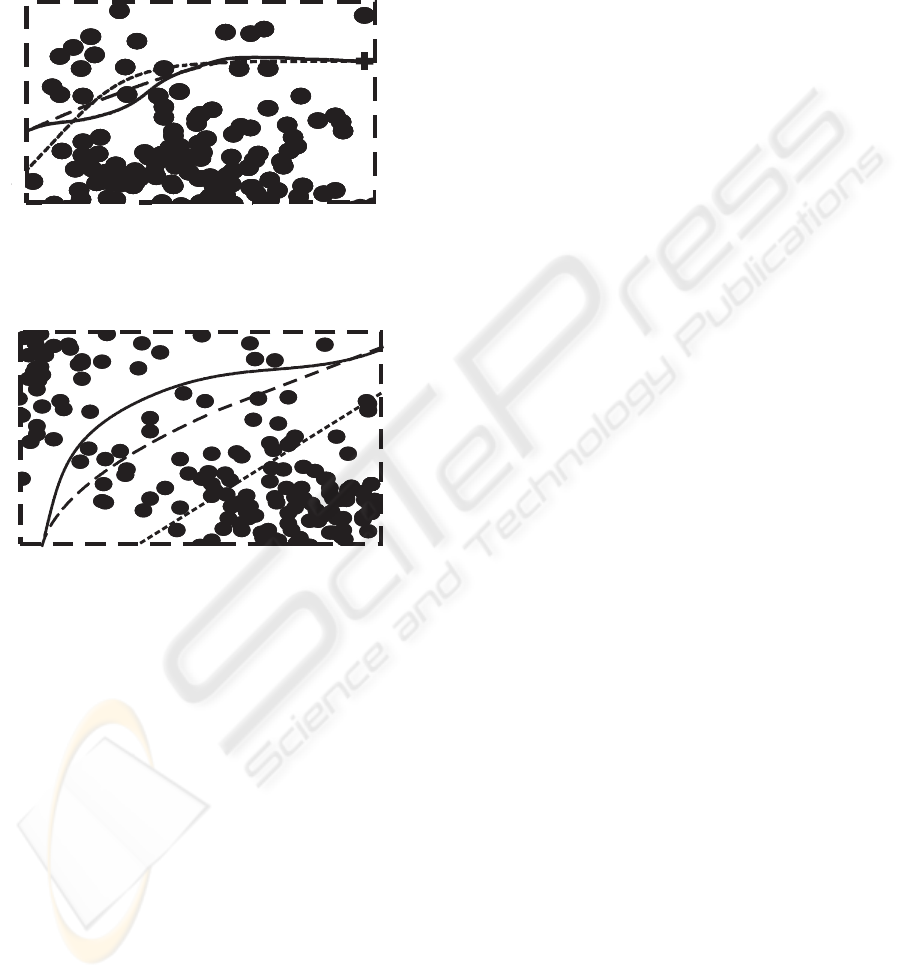
parameters is shown in Fig. 4. Looking at Fig. 5 and
6, the decreasing amount of collisions in the path at
different hierarchical levels can be observed. The so-
lution found in the first step (dotted line) contains 21
collisions along the whole path, but the control points
are situated far away from the obstacles and therefore
the big clusters are avoided. Only 4 collisions are con-
tained in the corrected path at the second level (dashed
line) and the final solution (solid line) after three hi-
erarchical optimizations is collision free.
In the second experiment the usage of the hierar-
chical method better agrees with a real application.
The stoping criterion now also considers the number
of collisions in the appropriate spline in addition to
the preset maximum hierarchical level. Collision free
parts of the solution do not need to be corrected in
the lower levels and thus the total number of itera-
tions is reduced. The maximum level as a part of the
stopping criterion is still important, because a colli-
sion free path may not exist and also a different fitness
function (equation 10) is applied in the lowest level.
Table 3 shows a comparison between the hierarchi-
ICINCO 2007 - International Conference on Informatics in Control, Automation and Robotics
120
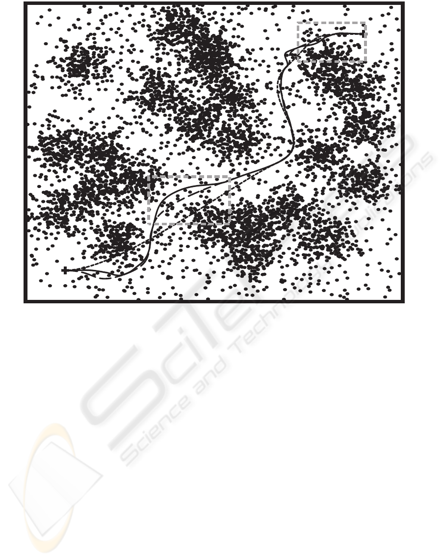
S
G
Figure 4: Situation with 3000 randomly generated obstacles. Dotted line - path found in the first level, dashed line - path
found in the second level, solid line - final solution found in the third level.
cal and the simple methods. The second row of the
table consists of the mean amount of iterations exe-
cuted by the PSO modules in the hierarchical algo-
rithm with different settings of the maximum level.
These values acted as inputs for the relevant runs of
the simple PSO algorithm that was run with different
numbers of splines (other parameters were set accord-
ing to (Saska et al., 2006b)).
The number of solutions that intersect with an ob-
stacle are displayed in the last four rows of the table.
Already in the third level, the presented hierarchical
approach achieved a result which is several times bet-
ter then the other algorithms. The computation reduc-
tion could be obtained, because the number of splines
was increased depending on the environment’s com-
plexity, but the size of the searched space remained
unchanged. The simple PSO method applied with a
number of populations lower than 300 obtained the
best results by using the shortest particle (only two
splines in the string). If the evolution process was
stopped after 1000 iterations, the optimal path was
composed of three splines. We suppose that the op-
timal length increases with the duration of the evolu-
tion, because a more complicated path allows to find
a collision free solution in the complex environment.
But due to the extension of the calculation time it is
not applicable in real time applications.
4 CONCLUSIONS AND FUTURE
WORK
In this paper a novel hierarchical path planning
method for complex environments was presented.
The developed algorithm is based on the optimization
of cubic splines connected to smooth paths. The fi-
nal solution is optimized by repeatedly used PSO for
collision parts of the path. The approach was inten-
sively verified in two experiments with 1000 random
generated situations. Each scenario, that was inspired
by a real environment, contained more than 2000 ob-
stacles.
The results of the experiments proved the ability
of the algorithm to solve the path planning task in
very complicated maps. Most of the testing situa-
tions were solved during the first five hierarchical lev-
els and therefore the first final path of the robot was
HIERARCHICAL SPLINE PATH PLANNING METHOD FOR COMPLEX ENVIRONMENTS
121
designed by only 5 runs of the PSO module (maxi-
mum 121 runs are necessary for the whole path). It
makes the algorithm usable in real time applications,
because the mission can be started already after 4 per-
cent of the total computational time and the rest of the
solution will be found during the robot’s movement.
G
Figure 5: Zoomed part of figure 4 close to the goal position.
Figure 6: Zoomed part of figure 4.
The optimal adjusted approach failed in the 6.5 per-
cent of the runs. In approximately 80 percent of these
unresolved situations a collision free solution did not
exist (due to unsuitable position of the random gen-
erated clusters) or could not be found during only
five hierarchical levels (part of the workspace was too
complicated). But error in 20 percent of the unre-
solved situations (about one percent of the total runs)
was caused by a placing of the control points near an
obstacle, in spite of the penalization p
inside
in the fit-
ness function 11. This problem can be solved using
constrained optimization methods (Parsopoulos and
Vrahatis, 2006),(Vaz and Fernandes, 2006), that guar-
antee fulfillment of the constrictions.
In future we would like to extend the algorithm to
be utilizable in dynamical environments. Only the rel-
evant part of the solution could be corrected due to
the decomposition of the total path. Other computa-
tional reduction could be achieved by using the old
cultivated population for the optimization of a partly
changed fitness function.
Also the stoping rules for the PSO module or for
the hierarchical sinking need to be improved. The cri-
teria should be combined with physical features of the
solution, because the fixed number of iterations and
levels must be determined for the specific situation.
Therewithal a superior solution can be obtained faster
by a more sophisticated setting of the PSO parame-
ters. Experiments showed that using the same values
of the constants in all levels is not the best solution
which gives scope for an innovation (Beielstein et al.,
2002).
Another stream will be focused on testing and
comparing different optimization methods (e.g. ge-
netic algorithms (Tu et al., 2003), simulated annealing
(Janabi-Sharifi and Vinke, 1993), (Martinez-Alfaro
and Gomez-Garcia, 1998) or ant colony (Liu et al.,
2006)). We also plan to adapt the PSO algorithm for
this special task. The main idea is to use the pleasant
feature of the Ferguson splines. The control points
lie on the path (opposite for example in the robotic
often used Coons curves (Faigl et al., 2006)) and so
it is possible to put the initial population for instance
on the shortest path in the Voronoi diagram (Auren-
hammer and Klein, 2000) or in the Transformed net
(Saska et al., 2006a). This innovation reduces the
computational time, because the exploratory mode of
the particle swarm optimization can be skipped.
ACKNOWLEDGEMENTS
This work was supported by the Elitenetwork of
Bavaria through the program ”Identification, Opti-
mization and Control with Applications in Modern
Technologies”.
REFERENCES
Aurenhammer, F. and Klein, R. (2000). Voronoi diagrams.
Hand book of Computational Geometry. Elsevier Sci-
ence Publishers, Amsterodam.
Azariadis, P. and Aspragathos, N. (2005). Obstacle
representation by bump-surface for optimal motion-
planning. Journal of Robotics and Autonomous Sys-
tems, 51/2-3:129–150.
Beielstein, T., Parsopoulos, K. E., and Vrahatis, M. N.
(2002). Tuning pso parameters through sensitivity
analysis. In Technical Report, Reihe Computational
Intelligence CI 124/02., Collaborative Research Cen-
ter (Sonderforschungsbereich) Department of Com-
puter Science, University of Dortmund.
Borenstein, J. and Koren, Y. (1991). The vector field his-
togram: Fast obstacle avoidance for mobile robots.
IEEE Journal of Robotics and Automation, 7(3):278–
288.
ICINCO 2007 - International Conference on Informatics in Control, Automation and Robotics
122

Eberhart, R. C. and Kennedy, J. (1995). A new optimizer
using particle swarm theory. In Proceedings of the
Sixth International Symposium on Micromachine and
Human Science., pages 39–43, Nagoya, Japan.
Faigl, J., Klacnar, G., Matko, D., and Kulich, M. (2006).
Path planning for multi-robot inspection task consid-
ering acceleration limits. In Proceedings of the four-
teenth International Electrotechnical and Computer
Science Conference ERK 2005, pages 138–141.
Franklin, W. R., Akman, V., and Verrilli, C. (1985). Voronoi
diagrams with barriers and on polyhedra for minimal
path planning. In Journal The Visual Computer, vol-
ume 1(4), pages 133–150. Springer Berlin.
Hess, M., Saska, M., and Schilling, K. (2006). Formation
driving using particle swarm optimization and reactive
obstacle avoidance. In Proceedings First IFAC Work-
shop on Multivehicle Systems (MVS’06), Salvador,
Brazil.
Janabi-Sharifi, F. and Vinke, D. (1993). Integration of the
artificial potential field approach with simulated an-
nealing for robot path planning. In Proceedings of 8th
IEEE International Symposium on Intelligent Control,
pages 536–41, Chicago, IL, USA.
Kennedy, J. and Eberhart, R. (1995). Particle swarm opti-
mization. In Proceedings International Conference on
Neural Networks IEEE, volume 4, pages 1942–1948.
Khatib, O. (1986). Real-time obstacle avoidance for manip-
ulators and mobile robots. In The International Jour-
nal of Robotics Research, volume 5, pages 90–98.
Kunigahalli, R. and Russell, J. (1994). Visibility graph ap-
proach to detailed path planning in cnc concrete place-
ment. In Automation and Robotics in Construction XI.
Elsevier.
Latombe, J.-C. (1996). Robot motion planning. KluverAca-
demic Publishers, fourth edition.
Liu, S., Mao, L., and Yu, J. (2006). Path planning based on
ant colony algorithm and distributed local navigation
for multi-robot systems. In Proceedings of IEEE In-
ternational Conference on Mechatronics and Automa-
tion, pages 1733–8, Luoyang, Henan, China.
Macas, M., Novak, D., and Lhotska, L. (2006). Particle
swarm optimization for hidden markov models with
application to intracranial pressure analysis. In Biosig-
nal 2006.
Martinez-Alfaro, H. and Gomez-Garcia, S. (1998). Mobile
robot path planning and tracking using simulated an-
nealing and fuzzy logic control. In Expert Systems
with Applications, volume 15, pages 421–9, Monter-
rey, Mexico. Elsevier Science Publishers.
Nearchou, A. (1998). Solving the inverse kinematics prob-
lem of redundant robots operating in complex envi-
ronments via a modified genetic algorithm. Journal of
Mechanism and Machine Theory, 33/3:273–292.
Parsopoulos, K. E. and Vrahatis, M. N. (2006). Parti-
cle swarm optimization method for constrained op-
timization problems. In Proceedings of the Euro-
International Symposium on Computational Intelli-
gence.
Saska, M., Kulich, M., Klan
ˇ
car, G., and Faigl, J. (2006a).
Transformed net - collision avoidance algorithm for
robotic soccer. In Proceedings 5th MATHMOD
Vienna- 5th Vienna Symposium on Mathematical
Modelling. Vienna: ARGESIM.
Saska, M., Macas, M., Preucil, L., and Lhotska, L. (2006b).
Robot path planning using partical swarm optimiza-
tion of ferguson splines. In Proc. of the 11th IEEE
International Conference on Emerging Technologies
and Factory Automation. ETFA 2006.
Tu, J., Yang, S., Elbs, M., and Hampel, S. (2003). Genetic
algorithm based path planning for a mobile robot.
In Proc. of the 2003 IEEE Intern. Conference on
Robotics and Automation, pages 1221–1226.
Vaz, A. I. F. and Fernandes, E. M. G. P. (2006). Optimiza-
tion of nonlinear constrained particle swarm. In Re-
search Journal of Vilnius Gediminas Technical Uni-
versity, volume 12(1), pages 30–36. Vilnius: Tech-
nika.
Ye, J. and Qu, R. (1999). Fairing of parametric cubic
splines. In Mathematical and Computer Modelling,
volume 30, pages 121–31. Elseviers.
HIERARCHICAL SPLINE PATH PLANNING METHOD FOR COMPLEX ENVIRONMENTS
123
