MAKING SENSOR NETWORKS INTELLIGENT

Peter Sapaty

Institute of Mathematical Machines & Systems, National Academy of Sciences

Glushkova Ave 42, Kiev 03187, Ukraine

Masanori Sugisaka

Department of Electrical and Electronic Engineering, Oita University

700 Oaza Dannoharu 870-1192 Japan

Joaquim Filipe

Departamento Sistemas e Informática, Escola Superior de Tecnologia de Setúbal

Setúbal 2910-761, Portugal

Keywords: Sensor networks, intelligent management, distributed scenario language, distributed interpreter, tracking

objects, hierarchical data fusion.

Abstract: A universal solution for management of dynamic sensor networks will be presented, covering both

networking and application layers. A network of intelligent modules, overlaying the sensor network,

collectively interprets mission scenarios in a special high-level language that can start from any nodes and

cover the network at runtime. The spreading scenarios are extremely compact, which may be useful for

energy saving communications. The code will be exhibited for distributed collection and fusion of sensor

data, also for tracking mobile targets by scattered and communicating sensors.

1 INTRODUCTION

Sensor networks are a sensing, computing and

communication infrastructure that allows us to

instrument, observe, and respond to phenomena in

the natural environment, and in our physical and

cyber infrastructure (Culler at al., 2004; Chong,

Kumar, 2003). The sensors themselves can range

from small passive microsensors to larger scale,

controllable platforms. Their computation and

communication infrastructure will be radically

different from that found in today's Internet-based

systems, reflecting the device- and application-

driven nature of these systems.

Of particular interest are wireless sensor

networks, WSN (Wireless; Zhao, Guibas, 2004)

consisting of spatially distributed autonomous

devices using sensors to cooperatively monitor

physical or environmental conditions, such as

temperature, sound, vibration, pressure, motion or

pollutants, at different locations. WSN, however,

have many additional problems in comparison to the

wired ones. The individual devices in WSN are

inherently resource constrained--they have limited

processing speed, storage capacity, and

communication bandwidth. These devices have

substantial processing capability in the aggregate,

but not individually, so we must combine their many

vantage points on the physical phenomena within the

network itself. In addition to one or more sensors,

each node in a sensor network is typically equipped

with a radio transceiver or other wireless

communications device, a small microcontroller, and

an energy source, usually a battery. The size of a

single sensor node can vary from shoebox-sized

nodes down to devices the size of grain of dust.

Typical applications of WSNs include

monitoring, tracking, and controlling. Some of the

specific applications are habitat monitoring, object

tracking, nuclear reactor controlling, fire detection,

Sapaty P., Sugisaka M. and Filipe J. (2007).

MAKING SENSOR NETWORKS INTELLIGENT.

In Proceedings of the Fourth International Conference on Informatics in Control, Automation and Robotics, pages 92-100

DOI: 10.5220/0001640200920100

 SciTePress

traffic monitoring, etc. In a typical application, a

WSN is scattered in a region where it is meant to

collect data through its sensor nodes. They could be

deployed in wilderness areas, where they would

remain for many years (monitoring some

environmental variable) without the need to

recharge/replace their power supplies. They could

form a perimeter about a property and monitor the

progression of intruders (passing information from

one node to the next). At present, there are many

uses for WSNs throughout the world.

In a wired network like the Internet, each router

connects to a specific set of other routers, forming a

routing graph. In WSNs, each node has a radio that

provides a set of communication links to nearby

nodes. By exchanging information, nodes can

discover their neighbors and perform a distributed

algorithm to determine how to route data according

to the application’s needs. Although physical

placement primarily determines connectivity,

variables such as obstructions, interference,

environmental factors, antenna orientation, and

mobility make determining connectivity a priori

difficult. Instead, the network discovers and adapts

to whatever connectivity is present.

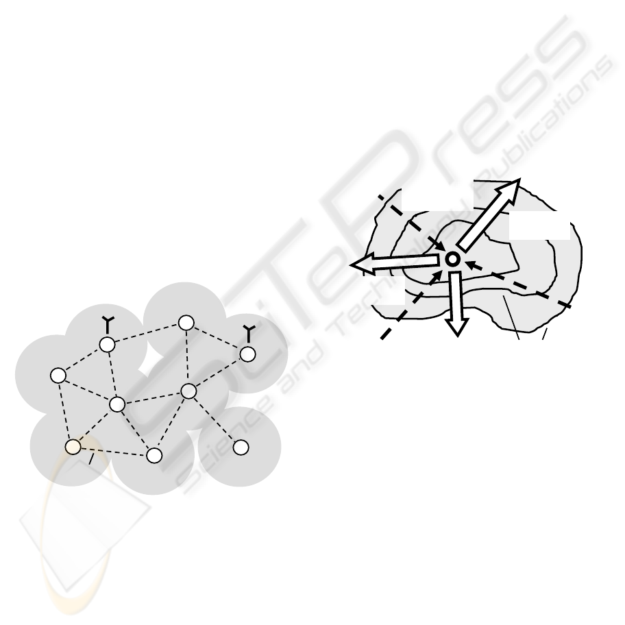
Fig. 1 shows what we will mean as a sensor

network for the rest of this paper.

Transmitter

Sensor

Local communication

capabilities

Figure 1: Distributed sensors and their emergent network.

It will hypothetically consist of (a great number of)

usual sensors with local communication capabilities,

and (a limited number of) those that can additionally

transmit collected information outside the area (say,

via satellite channels). Individual sensors can be on a

move, some may be destroyed while others added at

runtime (say, dropped from the air) to join the

existing ones in solving cooperatively distributed

problems.

The aim of this paper is to show how any

imaginable (or even so far unimaginable) distributed

problems can be solved by dynamic self-organized

sensor networks if to increase their intelligence as a

whole, with a novel distributed processing and

control ideology and technology effectively

operating in computer networks.

2 THE DISTRIBUTED

MANAGEMENT MODEL

The distributed information technology we are using

here is based on a special Distributed Scenario

Language (DSL) describing parallel solutions in

computer networks as a seamless spatial process

rather than the traditional collection and interaction

of parts (agents). Parallel scenarios in DSL can start

from any interpreter of the language, spreading and

covering the distributed space at runtime, as in Fig. 2.

Spreading

activities

Hierarchical

echoing and

control

Advances in space

Start

Spreading

activities

Figure 2: Runtime coverage of space by parallel scenarios.

The overall management of the evolving scenarios is

accomplished via the distributed track system

providing hierarchical command and control for

scenario execution, with a variety of special echo

messages. We will mention here only key features of

DSL, as the current language details can be found

elsewhere (Sapaty et al., 2007), also its basics from

the previous versions (Sapaty, 1999, 2005; Sapaty et

al., 2006).

A DSL program, or wave, is represented as one

or more constructs called moves (separated by a

comma) embraced by a rule, as follows:

wave → rule ({ move , })

Rules may serve as various supervisory, regulatory,

coordinating, integrating, navigating, and data

processing functions, operations or constraints over

moves.

MAKING SENSOR NETWORKS INTELLIGENT

A move can be a constant or variable, or

recursively an arbitrary wave itself:

move → constant | variable | wave

Variables classify as nodal, associated with space

positions and shared by different waves, frontal,

moving in space with program control, and

environmental, accessing the environment navigated.

Constants may reflect both information and physical

matter.

Wave, being applied in a certain position of the

distributed world, can perform proper actions in a

distributed space, terminating in the same or in other

positions. It provides final result that unites local

results in the positions (nodes) reached, and also

produces resultant control state. The (distributed)

result and the state can be subsequently used for

further data processing and decision making on

higher program levels. Parallel waves can start from

different nodes in parallel, possibly intersecting in

the common distributed space when evolving in it

independently.

If moves are ordered to advance in space one

after the other (which is defined by a proper rule),

each new move is applied in parallel in all the nodes

reached by the previous move. Different moves (by

other rules) can also apply independently from the

same node, reaching new nodes in parallel. The

functional style syntax shown above can express any

program in DSL, but if useful, other notations can be

used, like the infix one. For example, an

advancement in space can use period as operator

(separator) between successive steps, whereas

parallel actions starting from same node can be

separated by a semicolon. For improving readability,

spaces can be inserted in any places of the programs-

-they will be automatically removed before

execution (except when embraced by quotes).

The interpreter may have its own physical body

(say, in the form of mobile or humanoid robot), or

can be mounted on humans (like in mobile phones).

A network of the interpreters can be mobile and

open, changing its volume and structure, as robots or

humans can move at runtime. We will be assuming

for the rest of this paper that every sensor has the

DSL interpreter installed, which may have a

software implementation or can be a special

hardware chip.

In the following sections we will show and

explain the DSL code for a number of important

problems to be solved by advanced sensor networks,

which confirms an efficiency of the proposed

distributed computational and control model.

3 ELEMENTARY EXAMPLE

3.1 The Task

An elementary task to be programmed in DSL may

look like follows. Let it needs to go to the physical

locations of a disaster zone with coordinates (using

x-y pair here for simplicity) x25_y12, x40_y36, and

x55_y21, measure temperature there, and transmit

its value, together with exact coordinates of the

locations reached, to a collection center. The

corresponding program in DSL will be as follows:

Hop(x25_y12, x40_y36, x55_y21).

Transmit(Temperature & Location)

The program moves independently to the three

locations given, and in every destination reached

measures temperature using special environmental

variable Temperature. Using another

environmental variable Location, it attaches to

the previous value exact coordinates of the current

physical position (which, by using GPS, may differ

from the initially intended, rough coordinates). The

two-value results are then independently transmitted

from the three locations to a collection center.

This program reflects semantics of the task to be

performed in a distributed space, regardless of

possible equipment that can be used for this. The

latter may, for example, be a set of sensors scattered

in advance throughout the disaster zone, where

hopping by coordinates may result in a wireless

access of the sensors already present there--not

necessarily moving into these points physically. As

another solution, this program may task mobile

robots (single or a group) to move into these

locations in person and perform the needed

measurement and transmission upon reaching the

destinations.

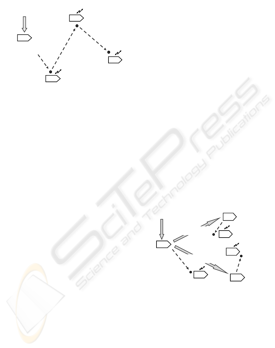
3.2 Single-Robot Solution

Let us consider how the previous program will be

executed with only a single robot available (let it be

Robot 1, assuming other robots not reachable). After

its injection into the robot’s interpreter (see Fig. 3),

the first, broadcasting statement:

Hop(x25_y12, x40_y36, x55_y21)

will be analyzed first. It naturally splits into three

independent hops, but only one can be performed at

the start by a single robot.

ICINCO 2007 - International Conference on Informatics in Control, Automation and Robotics

x25_y12

x55_y21

x40_y36

Hop(x25_y12, x40_y36,

x55_y21). Transmit

(Temperature &

Location)

Hop(x40_y36, x55_y21).

Transmit (Temperature

& Location)

Hop(x55_y21).

Transmit

(Temperature

& Location)

Robot 1

Transmit

(Temperature

& Location)

Program

injection

Hop(x25_y12, x40_y36, x55_y21).

Transmit(Temperature & Location)

Figure 3: Single-robot solution.

The interpreter hops virtually into the point

x25_y12 ordering robot to move into the

corresponding physical location. Upon arrival, the

second statement:

Transmit(Temperature & Location)

will be executed by measuring temperature,

attaching coordinates, and transmitting the result via

channels available. The rest of the program,

represented as:

Hop(x40_y36, x55_y21).

Transmit(Temperature & Location)

will be analyzed again, with hop to x40_y36

extracted, robot moved into the second location, and

measurement result transmitted as before. The

program’s remainder, now as:

Hop(x55_y21).

Transmit(Temperature & Location)

will cause movement and operation in the third

location x55_y21. The program terminates after

shrinking to:

Transmit(Temperature & Location)

All these steps are depicted detail in Fig. 3.

3.3 Multiple-Robot Solution

Let us consider now the case where other robots can

be requested and accessed from the robot into which

we injected our program (let it be Robot 1 again),

see Fig. 4. After analyzing the first statement,

splitting it into individual hops and attaching to each

of them the replicated rest of the program (i.e.

second statement) the interpreter in Robot 1 will

produce the following three independent programs:

Hop(x25_y12).

Transmit(Temperature & Location)

Hop(x40_y36).

Transmit(Temperature & Location)

Hop(x55_y21).

Transmit(Temperature & Location)

Leaving one of them (say, the first) for execution in

itself, Robot 1 requesting other available robots (let

them be Robot 2 and Robot 3) by a wireless channel

sends electronically the obtained other two programs

to them. After this, all three programs will be

operating in the three mentioned robots

independently and in parallel.

Each robot first executes the hop statement,

moving into the location given by physical

coordinates, and upon reaching the destination,

executes the second statement measuring

temperature and detecting exact coordinates,

subsequently transmitting these to the collection

center, exactly as for the previous case with a single

robot. All this is depicted in detail in Fig. 4.

x25_y12

x55_y21

x40_y36

Hop(x25_y12).

Transmit

(Temperature &

Location)

Transmit(Temperature

& Location)

Robot 1

Robot 2

Robot 1

Hop(x25_y12, x40_y36, x55_y21).

Transmit(Temperature & Location)

Transmit

(Temperature

& Location)

Transmit

(Temperature

& Location)

Hop(x55_y21). Transmit

(Temperature & Location)

Hop(x40_y36). Transmit

(Temperature & Location)

Initial

program

injection

Spreading

to other

robots

Robot 3

Robot 2

Robot 3

Figure 4: Multiple-robot solution.

The shown above were only elementary examples of

DSL code and rules of its execution. In other, more

complex cases DSL allows us to dynamically form

networked knowledge arbitrarily distributed between

dynamic resources, also providing hierarchical

control of distributed processes. DSL can provide

description of system missions on a semantic level,

with telling what, where, and why to do rather than

how and who should do this, effectively abstracting

from the resources (computer networks, robots,

MAKING SENSOR NETWORKS INTELLIGENT

humans) that can implement them, which can be

emergent and not known in advance. These

programs can be executed by any number of

technical or biological processors, where

organization of resources, their communication and

synchronization are delegated to efficient automatic

interpretation, with strict and simple implementation

rules.

Application programs in DSL are often hundreds

of times shorter than in conventional languages (like

C or Java). The DSL programs are interpreted rather

than compiled, adjusting to the execution

environment at runtime, which is especially

important when system components may be changed

or damaged during the execution. The approach is

based on the new, universal, formal system within

which any distributed and parallel algorithms can be

expressed and implemented.

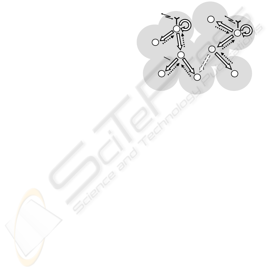
4 COLLECTING EVENTS

THROUGHOUT THE REGION

Starting from all transmitter nodes, the following

program regularly (with interval of 20 sec.) covers

stepwise, via local communications between sensors,

the whole sensor network with a spanning forest,

lifting information about observable events in each

node reached. Through this forest, by the internal

interpretation infrastructure, the lifted data in nodes

is moved and fused upwards the spanning trees, with

final results collected in transmitter nodes and sent

in parallel outside the system using rule Transmit

(See Fig. 5).

Hop(all transmitters).

Loop(

Sleep(20).

IDENTITY = TIME.

Transmit(

Fuse(

Repeat(free(observe(events));

Hop(directly reachable,

first come)))))

Globally looping in each transmitter node (rule

loop), the program repeatedly navigates (rule

repeat) the sensor set (possibly, in competition

with navigation started from other transmitters),

activating local space observation facilities in

parallel with the further navigation.

The resultant forest-like coverage is guaranteed

by allowing sensor nodes to be visited only once, on

the first arrival in them. The hierarchical fusion rule

fuse, collecting the scattered results, also removes

record duplicates, as the same event can be detected

by different sensors, leaving only most credible in

the final result. To distinguish each new global

navigation process from the previous one, it always

spreads with a new identity for which, for example,

current system time may be used (using

environmental variables IDENTITY and TIME of

the language).

Failed

Start

Fused

data

Global

loop

Global

loop

Repeated

parallel

navigation

Figure 5: Parallel navigation and data collection.

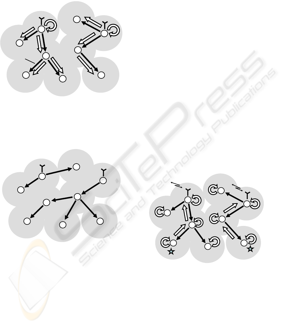
5 CREATING HIERARCHICAL

INFRASTRUCTURES

In the previous program, we created the whole

spanning forest for each global data collection loop,

which may be costly. To optimize this process, we

may first create a persistent forest infrastructure,

remembering which nodes were linked to which, and

then use it for a frequent regular collection and

fusion of the scattered data. As the sensor

neighborhood network may change over time, we

can make this persistent infrastructure changeable

too, updating it with some time interval (much larger,

however, than the data collection one), after

removing the previous infrastructure version. This

can be done by the following program that regularly

creates top-down oriented links named infra

starting from the transmitter nodes (as shown in Fig.

6).

Hop(all transmitters).

Loop(

Sleep(120).

IDENTITY = TIME.

Repeat(

Hop(directly reachable,

ICINCO 2007 - International Conference on Informatics in Control, Automation and Robotics

first come).

Remove links(all).

Stay(create link(-infra, BACK)))

infra

Persistent

links

Looping

updates

Looping

updates

Active

code

Figure 6: Runtime creation of hierarchical infrastructure.

This infrastructure creation program provides

competitive asynchronous spatial processes, so each

time even if the sensors do not change their positions,

the resultant infrastructure may differ, as in Fig. 7.

infra

Figure 7: Another possible infrastructure.

Having created a persistent infrastructure, we can

use it frequently by the event collection program,

which can be simplified now as follows:

Hop(all transmitters).

Loop(

Sleep(20).

Transmit(

Fuse(

Repeat(

Free(observe(events));

Hop(+infra)))))

The global infrastructure creation program (looping

rarely) and the event collection and fusion one

(looping frequently) can operate simultaneously,

with the first one guiding the latter on the data

collection routes, which may change over time.

6 ROUTING LOCAL EVENTS TO

TRANSMITTERS

We have considered above the collection of

distributed events in the top-down and bottom-up

mode, always with the initiative stemming from root

nodes of the hierarchy--the latter serving as a

parallel and distributed tree-structured computer. In

this section, we will show quite an opposite, fully

distributed solution, where each sensor node, being

an initiator itself, is regularly observing the vicinity

for the case an event of interest might occur.

Having discovered the event of interest, each

node independently from others launches a spatial

cyclic self-routing process via the infrastructure

links built before, which eventually reaches the

transmitter node, bringing with it the event

information, as shown in Fig. 8. The data brought to

the transmitters should be fused with the data

already existing there.

infra

Event

discovered

Event

discovered

Observing

Figure 8: Routing scattered events to transmitters.

The corresponding program will be as follows.

Hop(all nodes).

Frontal(Transfer).

Nodal(Result).

Loop(

Sleep(5).

Nonempty(

Transfer = observe(events)).

Repeat(hop(-infra)).

Result = Result & Transfer)

MAKING SENSOR NETWORKS INTELLIGENT

The transmitter nodes accumulating and fusing local

events, arriving from sensor nodes independently,

can subsequently send them outside the system.

Different strategies can be used here. For example,

one could be waiting until there are enough event

records collected in the transmitter before sending

them, and the other one waiting for a threshold time

and only then sending what was accumulated (if any

at all). The following program combines these two

cases within one solution, where arriving data from

sensors is accumulated in nodal variable Result.

Hop(all transmitters).

Loop(

Or(

Quantity(Result) >= 100,

(Sleep(60). Result != nil)).

Transmit(Result))

This program in every transmitter can work in

parallel with the previous program collecting events

and looping in every sensor (in transmitters as well,

assumed to be sensors too), and also with the earlier

program, starting in transmitters, for the regular

infrastructure updates.

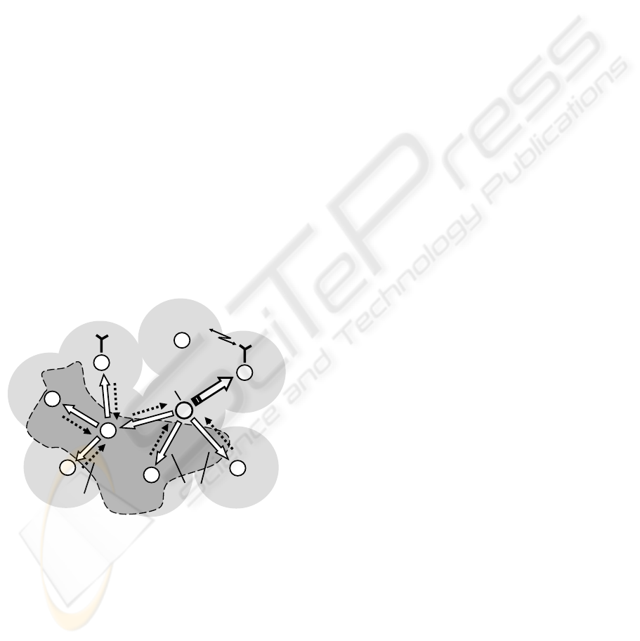
7 TRACKING MOBILE OBJECTS

Let us consider some basics of using DSL for

tracking mobile (say ground or aerial) objects

moving through a region controlled by

communicating sensors, as shown in Fig. 9. Each

sensor can handle only a limited part of space, so to

keep the whole observation continuous the object

seen should be handed over between the neighboring

sensors during its movement, along with the data

accumulated during its tracking and analysis.

The space-navigating power of the model

discussed can catch each object and accompany it

individually, moving between the interpreters in

different sensors, thus following the movement in

physical space via the virtual space (Sapaty, 1999).

This allows us to have an extremely compact and

integral solution unattainable by other approaches

based on communicating agents. The following

program, starting in all sensors, catches the object it

sees and follows it wherever it goes, if not seen from

the current point any more (more correctly: if its

visibility becomes lower than a given threshold).

Moving

object

Tracking mobile

intelligence

Looping

in nodes

Figure 9: Active tracking of a mobile object.

Hop(all nodes).

Frontal(Threshold) = 0.1.

Frontal(Object) = search(aerial).

Visibility(Object) > Threshold.

Repeat(

Loop(

Visibility(Object) > Threshold).

Maximum destination(

Hop(directly reachable).

Visibility(Object) > Threshold))

The program investigates the object’s visibility in all

neighboring sensors in parallel and moves control

along with program code and accumulated data to

the neighboring sensor seeing it best (if visibility

there exceeds the threshold given).

This was only a skeleton program in DSL,

showing the space tracing techniques for controlling

single physical objects. It can be extended to follow

collectively behaving groups of physical objects (say,

flocks of animals, mobile robots, or troops). The

spreading individual intelligences can cooperate in

the distributed sensor space, self-optimizing jointly

for the pursuit of global goals.

8 AVERAGING PARAMETERS

FROM A REGION

Let us consider how it could be possible to asses the

generalized situation in a distributed region given,

say, by a set of its border coordinates, in a fully

distributed way where sensors located in the region

communicate with direct neighbors only. Assume,

for example, that the data of interest is maximum

pollution level throughout the whole region (it may

also be temperature, pressure, radiation level, etc.)

together with coordinates of the location showing

ICINCO 2007 - International Conference on Informatics in Control, Automation and Robotics

this maximum.

The following program, starting in all sensors

located in the region, regularly measures the

pollution level in its vicinity, updates local

maximum and, by communication with direct

neighbors, attempts to increase the recorded

maximum there too. Eventually, after some time of

this purely local communication activity all sensors

will have the same maximum value registered in

them and corresponding to the maximum on the

whole region (see the overall organization in Fig.

10).

Nodal(Level, Max, Region).

Frontal(Transfer).

Region = region definition.

Hop(all nodes, Region).

Loop(

Or parallel(

Loop(

Sleep(5).

Level = measure(pollution).

Stay(Level > Max. Max=Level).

Transfer = Max.

Hop(directly reachable,Region).

Transfer > Max. Max=Transfer),

sleep(120)).

Level == Max.

Transfer = Max & WHERE.

Repeat(hop(-infra)).

Transmit(Transfer))

As there may be many sensors located in the region

of interest, we will need forwarding only a single

copy of this resultant maximum value to a

transmitter for an output. This can be achieved by

delegating this task only to the sensor whose

measured local value is equal to the accumulated

maximum in it, which corresponds to the overall

region’s maximum.

Having discovered that it is the leader (after a

certain time delay), such a sensor organizes repeated

movement to the nearest transmitter via the earlier

created virtual infrastructure, carrying the resultant

maximum value in frontal variable Transfer, and

sending it outside the system in the transmitter

reached, as shown in Fig. 10.

Similar, fully distributed, organization may be

introduced for finding averaged values, or even for

assembling the global picture of the whole region

with any details collected by individual sensors (the

latter may be costly, however, with a more practical

solution skeleton shown in the next section).

Generalized

result

Local communications

Self-routing

to transmitter

Region of interest

Emergent

leader

node

Figure 10: Distributed averaging with active routing.

9 ASSEMBLING FULL PICTURE

OF THE REGION

To collect details from some region via local sensors

and merge them into the whole picture could, in

principle, be possible via local single-level

exchanges only, as in the previous section, but the

amount of communications and data transfer as well

as time needed may be unacceptably high. We were

finding only a single value (maximum) via frequent

internode communications, with minimal code

length.

But for obtaining the detailed global picture of

the region or of some distributed phenomenon, we

may have to gradually paint (grow) this picture in

every sensor node simultaneously, with high

communication intensity between the nodes. Also,

there may be difficult to determine the completeness

of this picture staying in local sensors only. A higher

integrity and hierarchical process structuring may be

needed to see a distributed picture via the dispersed

sensors with limited visual capabilities and casual

communications.

Different higher-level approaches can be

proposed and expressed in DSL for this. We will

show only a possible skeleton with spanning tree

coverage of the distributed phenomenon and

hierarchical collection, merging, and fusing partial

results into the global picture. The latter will be

forwarded to the nearest transmitter via the

previously created infrastructure (using links

infra), as in Fig. 11.

Hop(random, all nodes,

detected(phenomenon)).

Loop(

Frontal(Full) = fuse(

MAKING SENSOR NETWORKS INTELLIGENT

Repeat(

Free(collect(phenomenon));

Hop(directly reachable,

first come,

detected(phenomenon)))).

Repeat(hop(-infra)).

Transmit(Full))

In the more complex situations, which can be

effectively programmed in DSL too, we may have a

number of simultaneously existing phenomena,

which can intersect in a distributed space. We may

also face combined phenomena integrating features

of different ones. The phenomena (like flocks of

birds, manned or unmanned groups or armies,

spreading fire or flooding) covering certain regions

may change in size and shape, they may also move

as a whole preserving internal organization, etc.

In the previous language versions (Sapaty, 1999,

2005; Sapaty et al., 2006), a variety of complex

topological problems in computer networks were

investigated and successfully programmed in a fully

distributed and parallel manner, which included

connectivity, graph patterns matching, weak and

strong components like articulation points and

cliques, also diameter and radius, optimum routing

tables, etc., as well as topological self-recovery after

indiscriminate damages (Sapaty, 1999).

Full

picture

Initiator

Self-routing

to transmitter

Active space

coverage

Echoed

partial results

Figure 11: Space coverage with global picture fusion.

10 CONCLUSIONS

We have presented a universal and flexible approach

of how to convert distributed sensor networks with

limited resources in nodes and casual

communications into a universal spatial machine

capable of not only collecting and forwarding data

but also solving complex computational and logical

problems as well as making autonomous decisions in

distributed environments.

The approach is based on quite a different type

of high-level language allowing us to represent

system solutions in the form of integral seamless

spatial processes navigating and covering

distributed worlds at runtime. This makes parallel

and distributed application programs extremely short,

which may be especially useful for the energy

saving communications between sensors.

The code compactness and simplicity are

achieved because most of traditional synchronization

and data or agent exchanges (which are also on a

high level, with minimum code sent) are shifted to

efficient automatic implementation, allowing us

concentrate on global strategies and global solutions

instead.

REFERENCES

Chong, C.-Y., Kumar, S. P., 2003. Sensor networks:

Evolution, opportunities, and challenges. Proc. of the

IEEE, Vol. 91, No. 8, August, pp.1247-1256.

Culler, D., Estrin, D., Srivastava, M., 2004. Overview of

sensor networks, Computer, August, pp.41-49, publ.

by the IEEE Computer Society.

Sapaty, P. S., 1999. Mobile Processing in Distributed and

Open Environments, John Wiley & Sons, ISBN:

0471195723, New York, February, 436p.

(www.amazon.com).

Sapaty, P. S., 2005. Ruling Distributed Dynamic Worlds,

John Wiley & Sons, New York, May, 256p, ISBN 0-

471-65575-9 (www.amazon.com).

Sapaty, P., Sugisaka, M., Finkelstein, R., Delgado-Frias, J.,

Mirenkov, N., 2006. Advanced IT support of crisis

relief missions. Journal of Emergency Management,

Vol.4, No.4, ISSN 1543-5865, July/August, pp.29-36

(www.emergencyjournal.com).

Sapaty, P., Morozov, A., Finkelstein, R., Sugisaka, M.,

Lambert, D., 2007. A new concept of flexible

organization for distributed robotized systems. Proc.

Twelfth International Symposium on Artificial Life and

Robotics (AROB 12th’07), Beppu, Japan, Jan 25-27,

8p.

Wireless sensor network. Wikipedia, the free encyclopedia,

www.wikipedia.org.

Zhao, F., Guibas, L., 2004. Wireless Sensor Networks: An

Information Processing Approach (The Morgan

Kaufmann Series in Networking). Morgan Kaufmann,

376p.

ICINCO 2007 - International Conference on Informatics in Control, Automation and Robotics

100