
TRACKING CONTROL DESIGN FOR A CLASS OF AFFINE MIMO
TAKAGI-SUGENO MODELS
Carlos Ari
˜
no
Department of Systems Engineering and Design, Jaume I University, Sos Baynat S/N, Castell
´
o de la Plana, Spain
Antonio Sala, Jose Luis Navarro
Department of Systems Engineering and Control, Universidad Politcnica de Valencia, Camino de Vera, 14, Valencia, Spain
Keywords:
Fuzzy control, affine Takagi-Sugeno models, local models, LMI, setpoint change.
Abstract:
When controlling Takagi-Sugeno fuzzy systems, verification of some sector conditions is usually assumed.
However, setpoint changes may alter the sector bounds. Alternatively, setpoint changes may be considered as
an offset addition in many cases, and hence affine Takagi-Sugeno models may be better suited to this problem.
This work discusses a nonconstant change of variable in order to carry out offset-ellimination in a class of
MIMO canonical affine Takagi-Sugeno models. Once the offset is cancelled, standard fuzzy control design
techniques can be applied for arbitrary setpoints. The canonical models studied use as state representation a
set of basic variables and their derivatives. Some examples are included to illustrate the procedure.
1 INTRODUCTION
In the last decade, design of fuzzy controllers based
on the so-called Takagi-Sugeno TS models (Takagi
and Sugeno, 1985) has reached maturity (Sala et al.,
2005). TS models express the behaviour of a sys-
tem via a convex interpolation of local (homoge-
neous) linear models, where the interpolation func-
tions are fuzzy membership functions with and add-
1 conditions. In particular, designs using the Lin-
ear Matrix Inequality framework (Tanaka and Wang,
2001; Guerra and Vermeiren, 2004) have become
widespread. Part of the success of such techniques
is due to the existence of systematic methodologies
for TS fuzzy identification (Takagi and Sugeno, 1985;
Tanaka and Wang, 2001; Babuska, 1998; Nelles et al.,
2000).
One particular characteristic of the mainstream TS
control design framework is that all of the local mod-
els must share the same equilibrium point, usually set
to x = 0 for convenience. This is not a severe problem,
as the identification procedures above referred need
only be applied with a constant change of variable,
used in the context of Taylor linearisation in control
design for decades. Once that change of variable is
carried out, global stability and performance regard-
ing reaching x = 0 from any initial conditions can be
proved. The reader is referred to (Tanaka and Wang,
2001; Guerra and Vermeiren, 2004) for details on the
methodology.
An affine structure for TS models was also origi-
nally addressed in (Takagi and Sugeno, 1985), which
considers local models without the shared equilib-
rium point. This structure, to be denoted as Takagi-
Sugeno-Offset (TSO) may originate either directly
from the identification process or when considering
tracking tasks with varying setpoints in ordinary TS
models. Indeed, in the latter case, the change of
variable needed to transform the new operating point
into x = 0 should involve changing the shape of the
membership functions and the parameters of the lo-
cal models. Otherwise, the resulting models lose the
shared equilibrium point.
The above mentioned control methodologies must
be adapted to TSO models. Some ideas appear
in (Kim and Kim, 2002; Johansson, 1999), where
quadratic Lyapunov functions and S-procedure LMIs
(Boyd et al., 1994) are used to prove stability of the
origin. However, setpoint changes are not considered,
and the division into ellipsoidal zones of the operat-
ing regime results in a cumbersome procedure which
involves considering the different regions of overlap
of the antecedent membership functions.
As an alternative, this paper presents a particular
248
Ariño C., Sala A. and Luis Navarro J. (2007).
TRACKING CONTROL DESIGN FOR A CLASS OF AFFINE MIMO TAKAGI-SUGENO MODELS.
In Proceedings of the Fourth International Conference on Informatics in Control, Automation and Robotics, pages 248-255
DOI: 10.5220/0001640702480255
Copyright
c
SciTePress

class of TSO fuzzy models stemming from a canon-
ical representation which, basically, takes the con-
trolled outputs and its derivatives as the chosen set
of state variables. This canonical representation has
a clear physical insight and stems from usual canon-
ical forms in linear and nonlinear systems (Antsak-
lis Panos and Michel Anthony, 1997; Slotine and Li,
1991).
Once the canonical TSO models are introduced,
an offset-removing transformation for state feedback
is discussed, which is the main result of this work.
The offset-removing transformation will allow to ex-
press the original TSO model as an ordinary TS form
on the transformed variables, enabling standard fuzzy
TS control design techniques to be used in such a sys-
tem.
The structure of the paper is as follows. Section
2 will present the definitions for the canonical TSO
framework. Section 3 will present results on the equi-
librium point of the canonical representation and the
main offset-removing transformation. Some exam-
ples illustrating the approach will be given in Section
4, and a conclusion section will close the paper.
2 CANONICAL TSO MODELS
In this section, basic definitions of the fuzzy systems
under study will be presented, which generalise the
classical Takagi-Sugeno fuzzy system used in most
current design techniques (Tanaka and Wang, 2001;
Guerra and Vermeiren, 2004; Sala et al., 2005) de-
scribed by
˙x =
n
∑
i=1
µ
i
(z)(A
i
x+ B
i
u)
∑
i
µ
i
(z) = 1 (1)
where z is assumed to be a set of accessible variables
which may include some or all of those ones compris-
ing the state vector x plus external scheduling ones,
and µ
i
(z) are denoted as antecedent membership func-
tions.
Definition 1 Canonical local model with offset
Let us have a system with p inputs, p outputs and n
states defined by:
˙x = A· x+ B· u+ R
y = C· x (2)
where the state vector is assumed to be partitioned
according to the following structure:
x = [x
11
x
12
...x
1r
1
x
21
x
22
...x
2r
2
... x
p1
x
p2
...x
pr
p
]
T
(3)
i.e., p blocks of size r
1
, ..., r
p
respectively, r
1
+ · · · +
r
p
= n, compatible with the block structure in matri-
ces A, B, C, R to be described below.
Let us define an auxiliary matrix with dimension
q× (q− 1) as:
T
q
= [0
(q−1)×1
I
q−1
] (4)
where I
q−1
denotes the identity matrix with size (q−
1) × (q − 1) and 0
(q−1)×1
the zero matrix with size
(q − 1) × 1. Also, the notation [ ]
s×t
will denote a
matrix with dimension s × t with arbitrary elements.
Then, matrices in (2) have the structure:
A =
T
r
1
0
(r
1
−1)×r
2
... 0
(r
1
−1)×r
p
[ ]
1×n
0
(r
2
−1)×r
1
T
r
2
... 0
(r
2
−1)×r
p
[ ]
1×n
...
0
(r
p
−1)×r
1
... 0
(r
p
−1)×r
p−1
T
r
1
[ ]
1×n
(5)
B =
0
(r
1
−1)×p
[ ]
1×p
0
(r
2
−1)×p
[ ]
1×p
.
.
.
0
(r
p
−1)×p
[ ]
1×p
(6)
C =
1
0
0
.
.
.
0
[ ]
p×(r
1
−1)
0
1
0
.
.
.
0
[ ]
p×(r
2
−1)
...
0
0
.
.
.
0
1
[ ]
p×(r
p
−1)
(7)
R =
0
(r
1
−1)×p
[ ]
1×p
0
(r
2
−1)×p
[ ]
1×p
.
.
.
0
(r
p
−1)×p
[ ]
1×p
(8)
Note 1 The above system structure is similar to
the well-known reachable canonical form (Antsak-
lis Panos and Michel Anthony, 1997). For instance,
a canonical SISO system:
A =
0 1 0 ... 0
0 0 1 ... 0
... ... ... ... ...
0 0 0 ... 1
−a
1
−a
2
−a
3
... −a
q
(9)
B =
0 0 0 ... b
T
(10)
TRACKING CONTROL DESIGN FOR A CLASS OF AFFINE MIMO TAKAGI-SUGENO MODELS
249

C =
1 c
2
c
3
... c
q
(11)
R =
0 0 0 ... r
T
(12)
conforms to the above structure.
Definition 2 Canonical Fuzzy Takagi-Sugeno-Offset
model.
A Fuzzy canonical Takagi-Sugeno-Offset model will
be defined according to the following structure:
˙x =
m
∑
i
µ
i
(z)(A
i
· x+ B
i
· u+ R
i
)
y =
m
∑
i
µ
i
(z)C
i
x (13)
where each of the component models has matrices A
i
,
B
i
, R
i
y C
i
which follow the structure in Definition
1 and µ
i
(z) are the membership functions, which are
assumed to verify
∑
i
µ
i
(z) = 1.
The notation below will be used as shorthand for
fuzzy summations
e
Ω(z) =
∑
i
µ
i
(z)Ω
i
(14)
Then, the fuzzy system in Definition 2 may be
written as:
˙x =
e
A(z) · x+
e
B(z) · u+
e
R(z)
y =
e
C(z)x (15)
by using
e
A(z) =
∑
n
i
µ
i
(z) · A
i
,
e
B(z) =
∑
n
i
µ
i
(z) · B
i
, etc.
3 OFFSET-ELLIMINATION
PROCEDURE
Proposition 1 Given a system with the structure in
Definition (1), for constant inputs u = u
eq
, the equi-
librium values of the state variables verify
x
eq
ij
= 0 i = 1, . . ., p j = 2, . . . , r
i
(16)
Proof: With u = u
eq
, the equilibrium equation is:
0 = Ax
eq
+ Bu
eq
+ R (17)
Using the canonical matrix structure, the states
x
i2
. . . x
ir
i
∀ i verify:
0
(r
i
−1)×1
=
I
(r
i
−1)×(r
i
−1)
x
eq
i2
.
.
.
x
eq
ir
i
+ 0
(r
i
−1)×p
u
eq
1
.
.
.
u
eq
p
+ 0
(r
i
−1)×1
(18)
Hence,
0 = I
(r
i
−1)×(r
i
−1)
·
x
eq
i2
.
.
.
x
eq
ir
i
i = 1, . . . , p (19)
finally obtaining (16).
Proposition 2 Given a system with the structure in
Definition 1, with constant input u = u
eq
, the equi-
librium values for the state vector and the output are
related, in the form:
x
eq
= [y
eq
1
0
1×(r
1
−1)
y
eq
2
0
1×(r
2
−1)
. . . y
eq
p
0
1×(r
1
−1)
]
T
y
eq
= [y
eq
1
. . . y
eq
p
]
T
Proof: Replacing x
eq
in the output equation,
y
eq
= C · x
eq
(20)
given the structure of C (7) and the results from the
previous proposition, stating that only the states cor-
responding to the columns of the identity may be
nonzero, we have:
y
eq
=
x
eq
11
x
eq
21
.
.
.
x
eq
p1
(21)
and finally,
x
eq
= [y
eq
1
0
1×(r
1
−1)
y
eq
2
0
1×(r
2
−1)
. . . y
eq
p
0
1×(r
p
−1)
]
T
Lemma 1 Given a canonical fuzzy system with the
structure in Definition 2, i.e.,
˙x =
e
A(z) · x+
e
B(z) · u+
e
R(z)
y =
e
C(z)x (22)
defining an auxiliary input
u
est
(z, y
ref
) =
(
e
C(z)
e
A(z)
−1
e
B(z))
−1
(−y
ref
−
e
C(z)
e
A(z)
−1
e
R(z)) (23)
under suitable invertibility assumptions, and carrying
out the change of variable
ˆx = x− x
ref
(24)
ˆu = u− u
est
(z, y
ref
) (25)
where
x
ref
= [y
ref,1
0
1×(r
1
−1)
y
ref,2
0
1×(r
2
−1)
. . .
. . . y
ref,p
0
1×(r
1
−1)
]
T
(26)
and
y
ref
= [y
ref,1
. . . y
ref,p
] (27)
ICINCO 2007 - International Conference on Informatics in Control, Automation and Robotics
250

is a user-defined vector, then ˆx = 0, ˆu = 0 is the new
equilibrium point for the system in the variables ˆx, ˆu
and, moreover, the transformed system has the equa-
tions:
˙
ˆx =
∑
i
µ
i
(z)(A
i
ˆx+ B
i
ˆx) (28)
i.e., it is a standard Takagi-Sugeno fuzzy system (1),
where the offset terms have dissapeared. The vari-
ables ˆx, ˆu will be denoted as incremental.
Proof:
Let us denote by S
z
0
the local affine system formed
by the result of evaluating
e
A,
e
B,
e
C and
e
R at a particular
(arbitrary) point z
0
:
˙
ξ =
e
A(z
0
) · ξ+
e
B(z
0
) · u+
e
R(z
0
)
y =
e
C(z
0
)ξ (29)
which has the canonical structure of definition (1).
Let us compute the input u
est
= u
est
(z
0
, y
ref
) so that
output y
ref
is an equilibrium point for the above sys-
tem S
z
0
, by using the equilibrium equation:
0 =
e
A(z
0
) · ξ
ref
+
e
B(z
0
) · u
est
+
e
R(z
0
) (30)
y
ref
=
e
C(z
0
) · ξ
ref
(31)
On the following the dependence on z
0
will be omit-
ted for notational simplicity. Carrying out some oper-
ations,
e
B· u
est
= −
e
A· ξ
ref
−
e
R
e
C
e
A
−1
e
B· u
est
= −
e
Cξ
ref
−
e
C
e
A
−1
e
R = −y
ref
−
e
C
e
A
−1
e
R
u
est
= (
e
C
e
A
−1
e
B)
−1
(−y
ref
−
e
C
e
A
−1
e
R) (32)
Let’s now obtain the equilibrium state ξ
ref
. Indeed,
as u
est
(z
0
, y
ref
) ensures that the output y
ref
is an equi-
librium point, and as S
z
0
has the structure 1, then
Proposition 2 ensures that ξ
ref
is:
ξ
ref
= [y
ref,1
0
1×r
1
y
ref,2
0
1×r
2
. . . y
ref,p
0
1×r
1
]
T
identical to the state x
ref
defined in (26). As z
0
in (30)
is an arbitrary point, then
0 =
e
A(z) · x
ref
+
e
B(z) · u
est
(z, y
ref
) +
e
R(z) ∀ z (33)
Carrying out the change of variable
ˆx = x− x
ref
ˆu = u− u
est
(z, y
ref
)
and using (33), the system equations may be written
as
˙x =
e
Ax+
e
Bu+
e
R =
e
Ax+
e
Bˆu+
e
Bu
est
+
e
R
˙x =
e
Ax+
e
Bˆu−
e
Ax
ref
−
e
R+
e
R =
e
A(x− x
ref
) +
e
Bˆu
˙x =
e
Aˆx+
e
Bˆu
If y
ref
is considered as a constant setpoint (˙y
ref
= 0) ,
then ˙x
ref
= 0 and, hence
˙
ˆx = ˙x. So the fuzzy system
in the new variables results in:
˙
ˆx =
e
Aˆx+
e
Bˆu =
∑
i
µ
i
(z)(A
i
ˆx+ B
i
ˆx)
whose equilibrium point is ˆx = 0, corresponding to
x
ref
(and output y
ref
) in the original non-incremental
variables.
The system in the new variables has its offset term re-
moved and a standard fuzzy controller may be designed on
it, such as the ones in (Tanaka and Wang, 2001) using LMI
techniques, which will be used in the examples below. The
control action for the original system will be computed by
adding to the resulting control action the term u
est
(z, y
ref
).
Note also that, with an ordinary TS system and a set-
point y = 0, the result is u
est
= 0, hence the proposed frame-
work encompasses the standard one. For the canonical sys-
tems, it is more powerful, however, as setpoint changes can
be immediately accommodated as the examples below will
illustrate.
4 EXAMPLES
In this section, a set of examples showing the possibilities
of the proposed approach will be presented. First, the con-
trol of a standard TS fuzzy system with no offset will be
extended to varying operation points, in order to compare
with the results applying usual methodologies involving a
constant change of variable. Then, a second example will
illustrate the proposed methodology in a MIMO case.
Example 1 Let us have a standard, offset-free system de-
fined by:
˙x =
2
∑
i=1
µ
i
(z)(A
i
x+ B
i
u)
y = Cx (34)
with the two models given by:
A
1
=
0 1 0
0 0 1
1 2 1
(35)
A
2
=
0 1 0
0 0 1
4 8 4
(36)
B
1
= B
2
=
0 0 1
T
(37)
C =
1 0 0
(38)
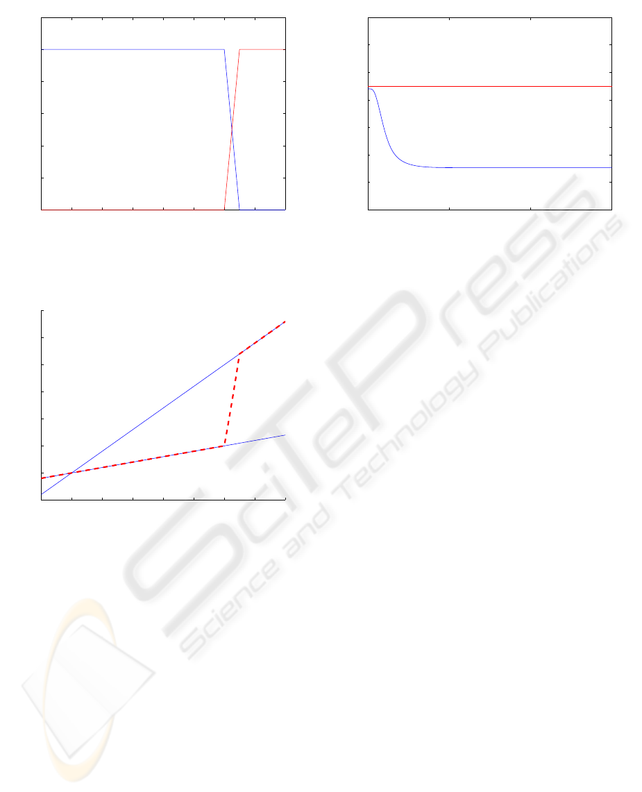
and membership functions µ
i
(z), defined on z = x
1
+
2x
2
+ x
3
as the trapezoidal partition depicted in Figure 1.
Figure 2 shows the nonlinearity in the system as a function
of z. Note that conditions to design a standard PDC con-
troller (Tanaka and Wang, 2001) for the TS system to reach
the origin are fulfilled. For instance, an LMI methodology
TRACKING CONTROL DESIGN FOR A CLASS OF AFFINE MIMO TAKAGI-SUGENO MODELS
251
−1 0 1 2 3 4 5 6 7
0
0.2
0.4
0.6
0.8
1
µ
1
µ
2
z
Figure 1: Membership functions.
−1 0 1 2 3 4 5 6 7
−5
0
5
10
15
20
25
30
A
2
A
1
z
˙x
3
− u
˜
A
Figure 2: Nonlinearity in ˙x
3
− u.
(Tanaka and Wang, 2001) may be applied. To achieve a
decay rate α, the following LMIs must be verified:
−XA
T
1
− A
1
X +M
T
1
B
T
1
+ B
1
M
1
− 2αX > 0 (39)
−XA
T
2
− A
2
X +M
T
2
B
T
2
+ B
2
M
2
− 2αX > 0 (40)
−XA
T
1
− A
1
X − XA
T
2
− A
2
X +M
T
1
B
T
2
+ (41)
+B
2
M
1
+ M
T
2
B
T
1
+ B
1
M
2
− 4αX > 0 (42)
where
X = P
−1
, M
1
= F
1
X, M
2
= F
2
X (43)
being P a quadratic matrix defining a Lyapunov function
and F
1
and F
2
the state feedback gains to be implemented,
i.e., the control action:
ˆu = −(µ
1
(z)F
1
+ µ
2
(z)F
2
) ˆx (44)
0 5 10 15
4.8
4.9
5
5.1
5.2
5.3
5.4
Y
Y
ref
t
Figure 3: System output Y.
A set of LMI conditions (decay α = 1) for the above
system yields the controller:
F
1
=
27.5203 28.7108 8.4221
(45)
F
2
=
30.5203 34.7108 11.4221
(46)
˜
F(z) =
2
∑
i=1
µ
i
(z)F
i
(47)
which, as expected, behaves correctly when reaching the
origin (figure not shown for brevity).
However, when trying to stabilise the system around a
new operating point (u
ref
= −13.125, y
ref
= 5.25, x
ref
=
(5.25, 0, 0)
T
), Lyapunov conditions no longer hold as the
linearised model at that point has slopes out of those given
by the vertices of the model above: in order to use a standard
methodology in that case, redefining the local models would
be needed. Indeed, with the constant change of variable
ˆu = u+ 13.125, ˆx = x− x
ref
(the usual one to achieve x = 0
as the operation point in many linear and fuzzy techniques),
the resulting controller
u = −13.125+
˜
F(z)(x− (5.25, 0, 0)
T
) (48)
yields an unstable equilibrium point: Figure 3 shows how
initial conditions in the vicinity of the desired target drift
away to another region of the state space.
On the contrary, the proposed methodology in this work
provides a controller valid for all operating points with no
modifications of the LMI conditions. Figure 4 shows the
non-constant u
est
calculated with lemma 1, which replaces
the constant value −13.125 in (48) above. In that way, the
resulting loop has the desired operating point as a stable
equilibrium with the desired decay rate, as shown in Figure
5.
Example 2 This example will demonstrate the methodol-
ogy on a 5th order MIMO Takagi-Sugeno-Offset system
with two unstable local models given by:
ICINCO 2007 - International Conference on Informatics in Control, Automation and Robotics
252
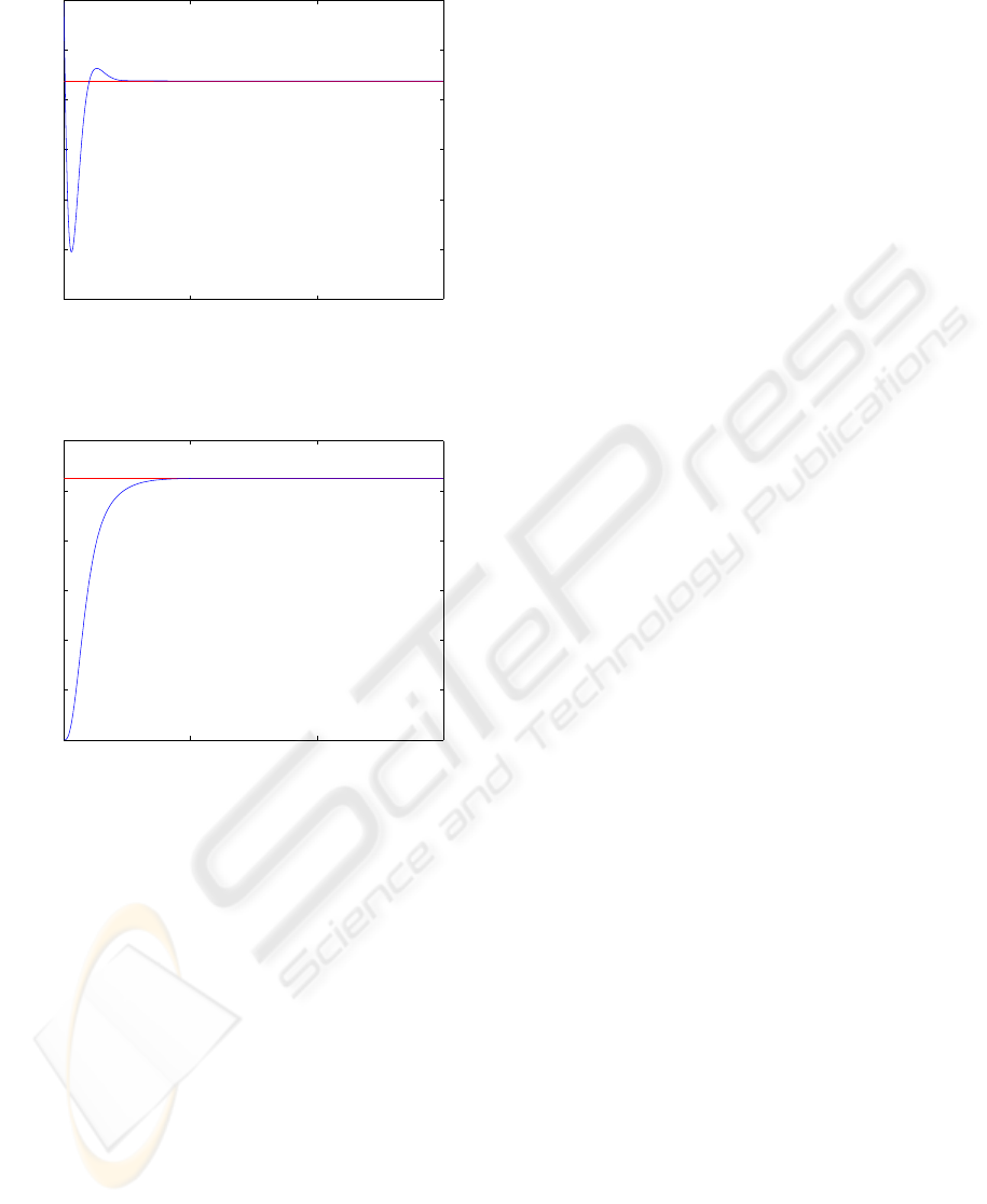
0 5 10 15
−14
−13.8
−13.6
−13.4
−13.2
−13
−12.8
U
est
t
Figure 4: Non-constant u
est
control action.
0 5 10 15
0
1
2
3
4
5
6
Y
Y
ref
t
Figure 5: System output Y with non-constant u
est
.
˙x =
2
∑
i=1
µ
i
(z)(A
i
(x− x
i0
) + B
i
(u− u
i0
))
y =
2
∑
i=1
µ
i
(z)C
i
x (49)
where
A
1
=
0 1 0 0 0
0 0 1 0 0
4 2 −5 3 0
0 0 0 0 1
1 −1 −5 −5 −1
(50)
B
1
=
0 0 2 0 1
0 0 1 0 0
T
(51)
A
2
=
0 1 0 0 0
0 0 1 0 0
5 1 0.1 2 0
0 0 0 0 1
1 −1 −1 −2 −1
(52)
B
2
=
0 0 10 0 1
0 0 1 0 0
T
(53)
C
1
=
1 0.1 0.05 0 −0.1
0 −0.2 0.5 1 −0.1
(54)
C
2
=
1 0.2 0.1 0 −0.2
0 −0.1 −0.5 1 0.2
(55)
x
10
=
0 0 0 0 0
T
(56)
u
10
=
0 0
T
(57)
x
20
=
2 0 0 2 0
T
(58)
u
20
=
1 3
T
(59)
and the membership functions µ
i
(z), defined on z = x
1
+ x
4
as:
µ
1
(z) =
1 z < 0
1− 0.25z 0 ≤ z ≤ 4
0 z > 4
(60)
being µ
2
(z) = 1− µ
1
(z).
Let us group the different equilibrium points of each
local model into an offset term:
R
i
= −A
i
x
i0
− B
i
u
i0
(61)
Hence, the system follows the structure in Definition 2. So
the control action u
est
(z, y
ref
), computed via (23), and the
equilibrium state are
x
ref
= [y
ref1
0 0 y
ref2
0]
T
(62)
u
est
= (
e
C
e
A
−1
e
B)
−1
(−y
ref
−
e
C
e
A
−1
e
R) (63)
where y
ref1
and y
ref2
are arbitrary user-defined setpoints
for the two plant outputs. As usual, the change of variable
removes the offset terms so the system may be expressed as
˙
ˆx =
∑
2
i=1
µ
i
(z)(A
i
ˆx+ B
i
ˆu). For a decay of α = 0.5, the LMI
Control Toolbox in Matlab obtains:
F
1
=
2.305 −1.104 −0.758 2.048 1.181
19.95 48.12 3.575 −22.27 −11.56
F
2
=
1.985 −1.718 −0.798 2.338 1.257
−0.792 45.89 12.89 −31.82 −15.57
Hence the actual control action to be applied to the
plant, after inverting the change of variable is:
u = u
est
(z, y
ref
)− (µ
1
(z)F
1
+µ
2
(z)F
2
)(x− x
ref
) (64)
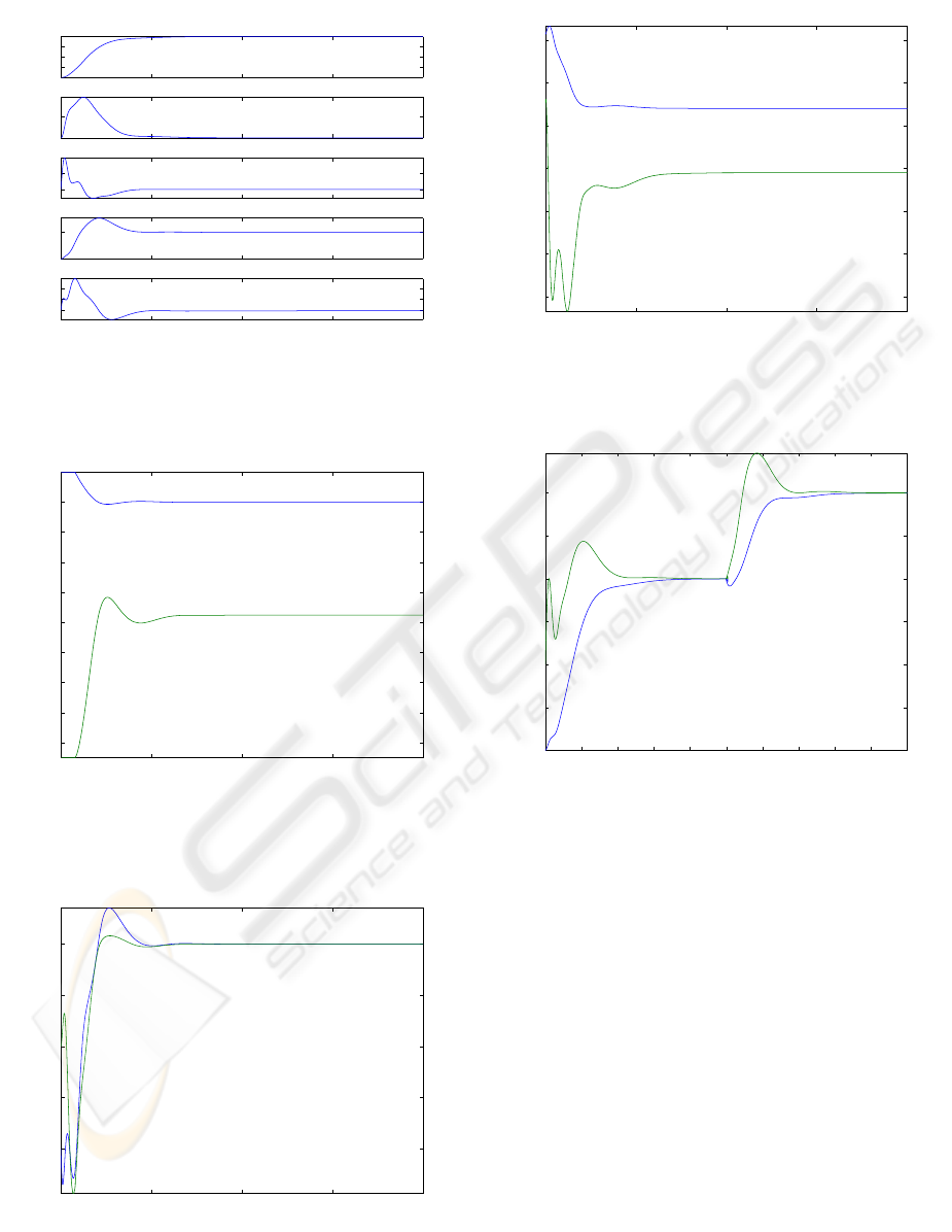
Figure 6 shows the system response approaching a
setpoint y
ref
= [1 1]
T
. The usefulness of the obtained
controller for setpoint changes is shown in Figure 10.
TRACKING CONTROL DESIGN FOR A CLASS OF AFFINE MIMO TAKAGI-SUGENO MODELS
253
0 5 10 15 20
−1
−0.5
0
0.5
0 5 10 15 20
0
0.5
0 5 10 15 20
0
1
2
0 5 10 15 20
0
1
0 5 10 15 20
0
0.5
1
x
1
x
2
x
3
x
4
x
5
t
Figure 6: Time response of the state variables.
0 5 10 15 20
−14
−12
−10
−8
−6
−4
−2
0
2
4
U
est1
U
est2
t
Figure 7: Offset removing term U
est
.
0 5 10 15 20
−1
−0.5
0
0.5
1
Y
1
Y
2
t
Figure 8: System output Y.
0 5 10 15 20
−20
−15
−10
−5
0
5
10
U
2
U
1
t
Figure 9: Actual overall control action U.
0 2 4 6 8 10 12 14 16 18 20
−1
−0.5
0
0.5
1
1.5
2
Y
1
Y
2
t
Figure 10: System outputY with a setpoint change toY
ref
=
(2, 2)
T
.
5 CONCLUSIONS
This paper presents an offset-ellimination change of
variable which applies to fuzzy Takagi-Sugeno-offset
models with local linear models with a particular
canonical structure. The canonical structure may be
obtained, for instance, by taking as state variables the
outputs and its derivatives.
As a result, a transformed system with equilibrium
at ˆx = 0 is obtained. The difference with standard
changes of variable is that it is non-constant in time.
As a result, the offset is neatly removed and the result-
ing transformed system has the same representation
for any desired setpoint, and well-known control de-
sign techniques for fuzzy non-offset Takagi-Sugeno
systems may be directly applied independently of the
ICINCO 2007 - International Conference on Informatics in Control, Automation and Robotics
254

chosen setpoint. Interestingly, as a particular case,
the procedure applies to setpoint changes in standard
offset-free Takagi-Sugeno models.
The presented results apply to a state feedback set-
ting. Further research should be devoted to generalis-
ing the procedure to situations with output feedback
and noisy measurements.
REFERENCES
Antsaklis Panos, J. and Michel Anthony, N. (1997). Linear
Systems. Ed. McGraw-Hill, New York, USA.
Babuska, R. (1998). Fuzzy Modeling for Control. Ed.
Kluwer Academic, Boston, USA.
Boyd, S., ElGhaoui, L., Feron, E., and Balakrishnan, V.
(1994). Linear matrix inequalities in system and con-
trol theory. Ed. SIAM, Philadelphia, USA.
Guerra, T. and Vermeiren, L. (2004). LMI-based re-
laxed nonquadratic stabilization conditions for nonlin-
ear systems in the Takagi-Sugeno’s form. Automatica,
40:823–829.
Johansson, M. (1999). Piecewise quadratic stability of
fuzzy systems. IEEE Trans. Fuzzy Syst., 7:713–722.
Kim, E. and Kim, S. (2002). Stabiliy analysis and synthe-
sis for affine fuzzy control system via LMI and ILMI:
Continous case. IEEE Transactions on Fuzzy Systems,
10:391–400.
Nelles, O., Fink, A., and Isermann, R. (2000). Local lin-
ear model trees (lolimot) toolbox for nonlinear system
identification. In Proc. 12th IFAC Symposium on Sys-
tem Identification. Elsevier.
Sala, A., Guerra, T., and Babuska, R. (2005). Perspectives
of fuzzy systems and control. Fuzzy Sets and Systems,
page In Print.
Slotine, J.-J. E. and Li, W. (1991). Applied Nonlinear Con-
trol. Ed. Prentice Hall, Englewood Cliffs,New Jersey.
Takagi, T. and Sugeno, M. (1985). Fuzzy identification of
systems and its applications to modeling and control.
IEEE Transactions on System, Man and Cybernetics,
15:116–132.
Tanaka, K. and Wang, H. O. (2001). Fuzzy control systems
design and analysis. Ed. John Wiley & Sons, New
York, USA.
TRACKING CONTROL DESIGN FOR A CLASS OF AFFINE MIMO TAKAGI-SUGENO MODELS
255
