A NEWMARK FMD SUB-CYCING ALGORITHM
J. C. Miao
(1,2)
, P. Zhu
(1)
, G. L. Shi
(1)
and G. L. Chen
(1)
School of Mechanical Engineering, Shanghai JiaoTong University, Shanghai, China
(1)
Department of Mechanical Engineering, Shazhou institute of technology, Zhangjiagang, China
(2)
Keywords: Flexible multi-body dynamics, Condensed FMD equation, Sub-cycling algorithm, Energy balance.
Abstract: This paper presents a Newmark method based sub-cycling algorithm, which is suitable for solving the
condensed flexible multi-body dynamic (FMD) problems. Common-step update formulations and sub-step
update formulations for quickly changing variables and slowly changing variables of the FMD are
established. Stability of the procedure is checked by checking energy balance status. Examples indicate that
the sub-cycling is able to enhance the computational efficiency without dropping results accuracy greatly.
1 INTRODUCTION
Flexible multi-body system (FMS) can be applied in
various domains such as space flight, automobiles
and robots. In these domains, accurate and efficient
computation of the flexible bodies undergoing large
overall motion is important for design and control of
the system (Huang and Shao, 1996).
Conventional integration methods, such as the
Newmark algorithm, the Runge-Kutta algorithm and
the Gear algorithm and etc (Dan Negrut, et al, 2005),
were widely applied to solve FMD equations.
Sub-cycling was proposed by Belytschko T. et al
(Belytschko T.,1978). Mark et al (Mark, 1989)
applied the method to simulate an impact problem
and computational cost of the sub-cycling was only
15% of that without sub-cycling. Gao H et al. (Gao,
2005) used sub-cycling to simulate auto-body
crashworthiness and declared that the cost is only
39.3% of no sub-cycling. Tamer et al (Tamer, 2003)
pointed out that the FMD sub-cycling methods have
not yet been presented in literatures.
2 SUB-CYCLING FOR FMD
A sub-cycling is constituted by two types of cycles,
main-cycle and sub-cycle. The key for sub-cycling is
to appropriately treat with interactions of nodes on
the interface (Daniel, 1997).
2.1 Condensed Model of FMD
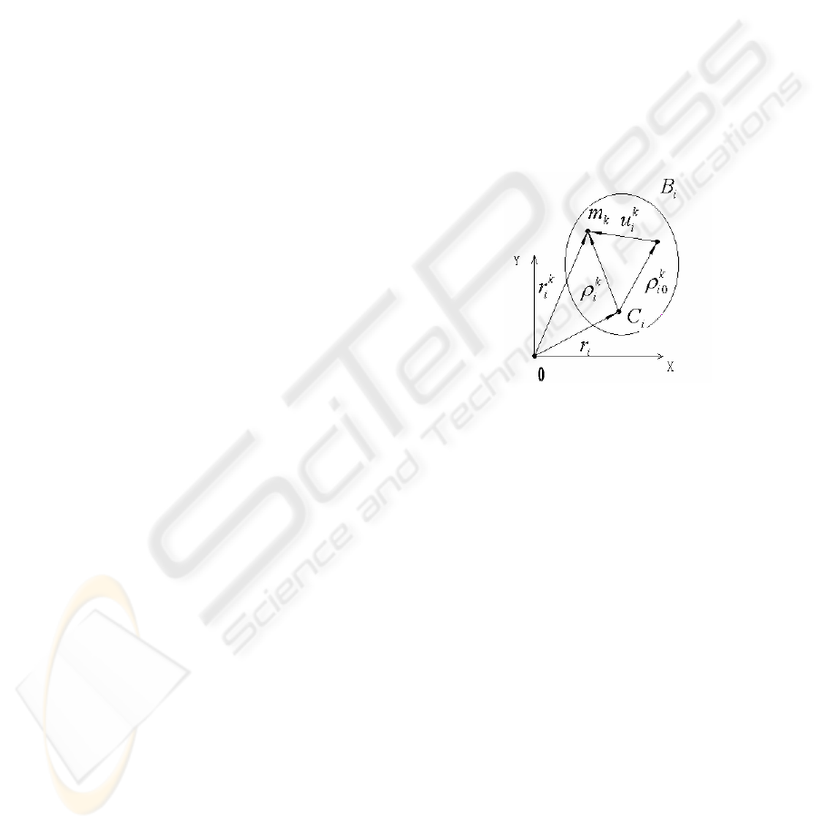
A flexible body is displayed in figure 1. Definition
of variables can be referenced in the literature (Lu,
1996).
Figure 1: A spatial arbitrary flexible body.
The FMD equation can be established by means
of the Lagrange formation.
()
)22(0,
)12(
−=
−+=++
""""""""
"

t
T
qC
QQλCKqqM
vFq
Thereinto, M is a general mass matrix, K is a
general stiffness matrix, C(q,t) is the constrains, Q
F
and Q
V
are general external load and general
centrifugal load. Λ is the Lagrange multiplier. By
means of two times of differentials of the constrain
equation, an augmented FMD equation can be
obtained as below.
)32( −
⎥
⎦
⎤
⎢
⎣
⎡
=
⎥
⎦
⎤
⎢
⎣
⎡
⎥
⎥
⎦
⎤
⎢
⎢
⎣
⎡
∗
"""

C
F
q
qr
Q
Q
λ
q
0C
CM
T
Due to the constraints, variables in (2-3) are
independent. By decomposition, a condensed FMD
equation can be established as following (Haug,
1989).
207
C. Miao J., Zhu P., L. Shi G. and L. Chen G. (2007).
A NEWMARK FMD SUB-CYCING ALGORITHM.
In Proceedings of the Fourth International Conference on Informatics in Control, Automation and Robotics, pages 207-211
DOI: 10.5220/0001641402070211
Copyright
c
 SciTePress

()
(
)
)42(,,,,
ˆ
,,
ˆ
−= "

tt
ddiiiidii
qqqqQqqqM
Thereinto:
() []
() []
γCMQCCγCMQQ
CCMMCCCCMMM
qFqqqF
qqqqqq
1*11*
111
ˆ
ˆ
−−−
−−−
−−−=
−−−=
ddid
idddid
ddd
T
T
idii
dddi
T
T
idiii
Equation（2-4） is a pure differential formation.
It is suitable for sub-cycling (Lu, 1996).
2.2 Newmark Integration for FMD
The Newmark integration is as following. There, q
t
denotes value of the general variable at time t. Δ t is
the step size.
β and γ are adjustable parameters.
[]
[]
2
(1 2 ) 2 (2 5)
2
(1 ) (2 6)
tt t t t tt
tt t t tt
t
t
t
ββ
γγ
+Δ +Δ
+Δ +Δ
Δ
=+Δ+ − + −
=+Δ − + −
qqq q q
qq qq

"
 
""""""
Define symbols below.
()
tata
t
aa
a
t
a
t
a
t
a
Δ=−Δ=
⎟
⎟
⎠
⎞
⎜
⎜
⎝
⎛
−
Δ
=−=
−=
Δ
=
Δ
=
Δ
=
γγ
β
γ
β
γ
βββ
γ
β
7654
321
2
0
12
2
1
1
2
111
The dynamic equation at time t+ Δ t can be
established below.
()
(
)
[]
()
)72(,,,
ˆ
,
ˆ
)1()1()1()1(
320
−=
−−−
Δ+Δ+Δ+Δ+
Δ+Δ+Δ+
"


tt
d
tt
d
tt
i
tt
ii
t
i
t
i
t
i
tt
i
tt
d
tt
ii
aaa
qqqqQ
qqqqqqM
Finally, we can get the results.
[]
)82(
ˆ
ˆ
0
3
0
2
1
0
−+++=
Δ+
−
Δ+Δ+
"

t
i
t
i
t
i
tt
i
tt
i
tt
i
a
a
a
a
a qqqQMq
Equation (2-8) need be solved iteratively. The
iteration process is as following.
1
() ( 1) ( 1)
0
3
2
00
ˆ
ˆ
(2 9)
ktt k tt k tt
iiii
ttt
iii
a
a
a
aa
−
+Δ − +Δ − +Δ
⎡⎤
=
⎣⎦
++ + −
qMQ
qqq

"
Thereinto, the top left corner marks represent the
number of the iteration step. Start-up initialisation of
iteration can be set-up below.
[]
)102(2)21(
2
)1(
2
)1(
−+−
Δ
+Δ+=
Δ+Δ+
"

ttttttt
t
t qqqqq
ββ
2.3 Newmark Sub-cycling for FMD
For simplification, all variables are separated into
two categories. The smaller step size is set to be Δ t.
The larger step size is set to be nΔ t. n is a positive
integer. Thus,
q

is expressed as a decomposed
format. And the condensed FMD formula can be
decomposed as a block matrix format as following.
)122(
ˆ
ˆ
ˆˆ
ˆˆ
−
⎥
⎥
⎦
⎤
⎢
⎢
⎣
⎡
=
⎥
⎦
⎤
⎢
⎣
⎡
⎥
⎥
⎦
⎤
⎢
⎢
⎣
⎡
"


t
S
t
L
S
L
t
SS
t
SL
t
LS
t
LL
Q
Q
q
q
MM
MM
The subscript symbol, L and S, represent the
larger step size and the smaller step size. M and Q
are the general mass matrix and the general external
force. According to balance status of the FMS at t+
Δ t and t+nΔ t, two groups of equations can be
obtained as following.
11 11 1
ˆ
ˆˆ
(2 13)
ˆ
ˆˆ
(2 14)
LLn Ln LSn Sn Ln
SL L SS S S
+= −
+= −
Mq Mq Q
Mq Mq Q
 
"
 
"
Thereinto,
Ln
q

and
Sn
q

are accelerations at
tnt
Δ
+
.
1L
q

and
1S
q

are accelerations at tt
Δ
+
.
The general mass matrix and the general external
force are defined similarly. Define symbols below.
1
333
1
3
1
2
22
1
2
2
1
0
00
1
0
,,,,, aaaa
n
a
aaa
n
a
aaa
nnn
======
In order to compute interaction between the
coupling variables at the common update, q
Sn
and
q
L1
need be estimated simultaneously. Similar to the
method (Daniel, 1997), q
L1
can be linearly
interpolated and q
Sn
can be linearly extrapolated by
means of the trapezoid rule. The formats of the
interpolations are expressed below.
()
10
00
11
(2 15)
(2 16)
LLLn
Sn Sn S S
n
nn
n
−
=+ −
=−+ −
qqq
qqqq
""""
"""
ICINCO 2007 - International Conference on Informatics in Control, Automation and Robotics
208

Hence action of the slowly changing variables to
the rapidly changing variables is calculated below.
() )172(
ˆ
0
1
30
1
20
1
0
11
−
⎥
⎦
⎤
⎢
⎣
⎡
−−−=− "

LLLLnSLSL
aa
n
a
qqqqMF
The action of the rapidly changing variables to
the slowly changing variables is calculated below.
() []
)182(
ˆ
0001
320
−−−−=− "

S
n
S
n
SS
n
LSnLSn
aaqna qqqMF
Imposing equations (2-17) and (2-18) into
equations (2-13) and (2-14), and co-multiplying a
number, n, to the left hand and the right hand of
equation (2-13), the common update formula of the
slowly changing variables and the rapidly changing
variables can be obtained below.
)192(
ˆˆ
ˆˆ
ˆˆ
ˆˆ
ˆˆ
ˆˆ
ˆ
ˆ
ˆˆ
ˆˆ
0
011
3
0
011
2
0
0
11
0
1
1
11
0
−
⎥
⎦
⎤
⎢
⎣
⎡
⎥
⎥
⎦
⎤
⎢
⎢
⎣
⎡
+
⎥
⎦
⎤
⎢
⎣
⎡
⎥
⎥
⎦
⎤
⎢
⎢
⎣
⎡
+
⎥
⎥
⎥
⎦
⎤
⎢
⎢
⎢
⎣
⎡
⎥
⎥
⎦
⎤
⎢
⎢
⎣
⎡
+
⎥
⎥
⎦
⎤
⎢
⎢
⎣
⎡
=
⎥
⎥
⎥
⎦
⎤
⎢
⎢
⎢
⎣
⎡
⎥
⎥
⎦
⎤
⎢
⎢
⎣
⎡
"




L
S
LLnLSn
SlSS
L
S
LLnLSn
SlSS
L
S
LLnLSn
SlSS
Ln
S
Ln
S
LLnLSn
SlSS
nn
aa
n
a
n
n
a
q
q
MM
MM
q
q
MM
MM
q
q
MM
MM
Q
Q
q
q
MM
MM
In order to get the sub-step update formula, the
following equation need be calculated at t+（i+1）
Δ t，i=1,2…(n-2).
)202(
ˆ
ˆˆ
)1()1()1()1()1(
−=+
+++++
"

iSiSiSSiLiSL
QqMqM
Also, according to equation (2-7), the following
equation can be obtained.
(
)
()
111
(1) 0 (1) 2 3
111
(1) 0 (1) 2 3 (1)
ˆ
ˆ
ˆ
(2 21)
SL i L i Li Li Li
SSi SiSi SiSiSi
aaa
aaa
++
++ +
⎡⎤
−− − +
⎣⎦
⎡⎤
−− − = −
⎣⎦
Mqqqq
MqqqqQ


"
In equation (2-21), the slowly changing variables,
which are used to compute the interaction of the
coupling variables, can be linearly interpolated in
terms of the trapezoid rule.
)232(
)222(
0
0
−+
−
=
−+
−
=
"""""

"""""
LnLL
LnLLi
n
i
n
in
n
i
n
in
i
qqq
qqq
In terms of equations (2-22) and (2-23), the
action of the slowly changing variables to the
rapidly changing variables can be approximately
assessed.
()
[
()()
()
()
()
(1) 0 0 2 0
1
1
30
1
ˆ
(
(2 24)
SL i Ln L L Ln
SL i
LLn
aanii
n
ani i
+
+
−= −−−+
⎤
−−+ −
⎦
FM qq qq
qq

 
"""" """
Imposing equation (2-24) into equation (2-21),
the sub-step update format can be got as following.
(
)
() ()
()
()
()
0(1)(1) (1) (1)0 2 3
0
2
(1) 0 (1) 0
1
3
(1) 0
ˆ
ˆˆ
ˆˆ
ˆ
(2 25)
SS i S i S i SS i Si Si Si
SL i Ln L SL i L Ln
SL i L Ln
aaaa
a
a
ni i
nn
a
ni i
n
++ + +
++
+
=+ ++
−−+−+
+−+ −
Mq Q M qqq
Mqq M qq
Mqq


 
""""" "
The energy balance status can be calculated by
means of the equation below (Mark and Belytschko,
1989).
)262(
int
−≤−+ ""WWWW
ext
nn
kin
n
δ
Thereinto, W
n
ext
is the work of the external forces
at nΔ t. W
n
int
is the internal energy at nΔ t. W
n
kin
is
the kinetic energy of the system at nΔ t.
δ is the
available error coefficient.
3 NUMERICAL EXAMPLES
In this section, two numerical examples will be
performed to validate availability and efficiency of
the present sub-cycling algorithm.
3.1 A Bar-slider System
A bar-slider system is shown in figure 2. Mass of the
rod is 2.0 kilograms and mass of the slider is 5.0
kilograms. The driving torque is 100 Nm/s. Stiffness
of the spring is 1000 N/m. length of the rigid rod is 2
meters.
Results of rotational angle of the rod, the
vibration amplification of the sliding block and the
energy balance status computed by means of the
sub-cycling and without sub-cycling are shown in
figure 3 to figure 6. The scale values in brackets of
the figure captions, such as (5:1), represent a sub-
cycling with 5 sub-steps in one major step.
A NEWMARK FMD SUB-CYCING ALGORITHM
209

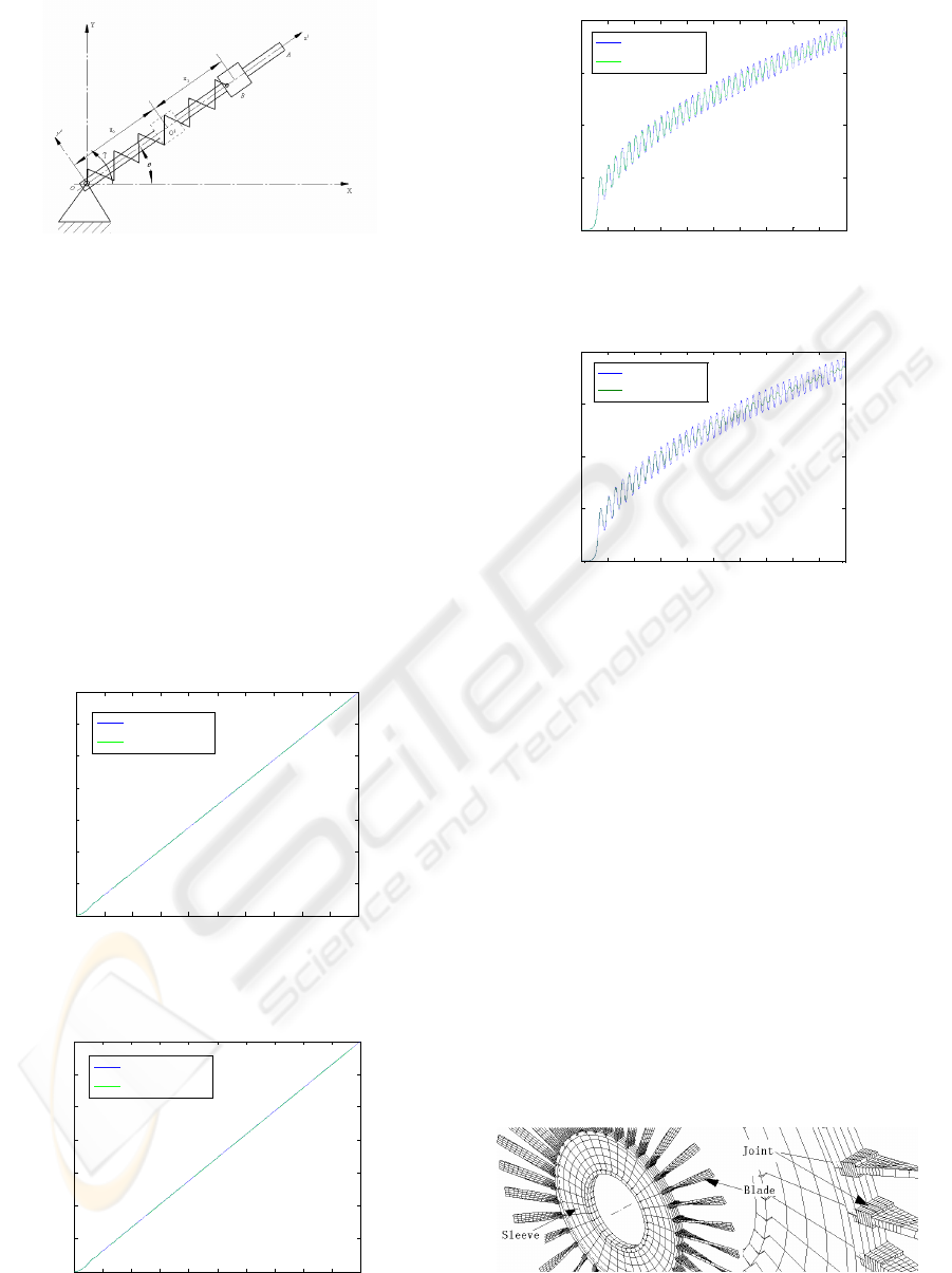
Figure 2: Rotational rod-spring-slider system.
Comparing the results in figure 3 to figure 6, we can
see that no matter which scale of the sub-cycling is
adopted, the results are very similar. The error of
sub-cycling with scale 10:1 is a little larger than that
of sub-cycling with scale 5:1. Yet all these two
errors are very small if compare with the original
results. The time cost of sub-cycling with scale 5:1
is 118 seconds and the time cost of the original
algorithm without sub-cycling is 218 seconds. The
proportion of time cost of these two algorithms is
54%. The time cost of sub cycling with scale 10:1 is
44 seconds and the proportion of time cost is only
20.2%. The results of balance checking illustrate that
the sub-cycling is stable during the integral process.
0 1 2 3 4 5 6 7 8 9 10
0
20
40
60
80
100
120
140
Time(s)
Rotational angle(radian)
no subcycling
subcycling
Figure 3: Rotational angle of the bar (5:1).
0 1 2 3 4 5 6 7 8 9 10
0
20
40
60
80
100
120
140
Time(s)
Rotational angle(radian)
no subcycling
subcycling
Figure 4: Rotational angle of the bar (10:1).
0 1 2 3 4 5 6 7 8 9 10
0
1
2
3
4
Time(s)
Amplification(m)
no subcycling
subcycling
Figure 5: Vibration amplification of the slider (5:1).
0 1 2 3 4 5 6 7 8 9 10
0
1
2
3
4
Time(s)
Amplification(m)
no subcycling
subcycling
Figure 6: Vibration amplification of the slider (10:1).
3.2 Airscrew of a Jet Engine
FEM model of the airscrew of a jet engine are
displayed in figure 7. Parameters of the model are as
following (Units: kg/N/mm/s). The material of
airscrew is aluminium alloy. EX=7e6, PR=3,
DEN=2.78e-6. Diameter of the airscrew is D=900
mm, rotate speed is 8000 rpm.
We simulate the large range overall motion of
the airscrew by means of the Newmark sub-cycling
and the original Newmark respectively. The
dynamic stress at the blade root is described in
figure 8. The time cost of the Newmark sub-cycling
is 1660 seconds and that of the Newmark is 2810
seconds. The computational efficiency is enhanced
about 70%. The compared results show the good
precision and stability of the Newmark sub-cycling.
Figure 7: The FEM model and the local mesh.
ICINCO 2007 - International Conference on Informatics in Control, Automation and Robotics
210

0 0.005 0.01 0.015 0.02
40
50
60
70
80
Time(s)
Dynamic stress(MPa)
no subcycling
subcycling
Figure 8: Dynamic stress of the blade root during rotation.
0 0.005 0.01 0.015 0.02
0
2
4
6
8
10
Time(s)
Rotational angle(radian)
no subcycling
subcycling
Figure 9: Rotational angle of the blade root.
4 CONCLUSIONS
This paper firstly presents a Newmark-based FMD
sub-cycling algorithm. By modifying the Newmark
integral formula to be fitted for sub-cycling of the
FMD problems, not only the integral efficiency can
be greatly improved, but also be more easy for
convergence of the integral process.
Because of that different integral step sizes are
adopted during the sub-cycling, the integral process
can be more efficient and easier for convergence. At
the same time, Unconditional stability of the original
Newmark are still kept in the Newmark sub-cycling.
The number of the sub-step in one major cycle
can be a little infection of the integral precision of a
sub-cycling process. However, it is unobvious as the
number is within a range. Generally speaking, the
enhancement of the integral efficiency is more
significant when the number is under a limitation.
By checking the energy balance status of the
integral process real time and adjusting the step size
when necessary, the sub-cycling procedure can keep
a well convergence property and obtain the
reasonable numerical computation results.
REFERENCES
Huang Wenhu, Shao Chengxun, 1996. Flexible multi-body
dynamics, The science Press.
Dan Negrut, Jose L, Ortiz., 2005. On an approach for the
linearization of the differential algebraic equations of
multi-body dynamics. Proceedings of IDETC/MESA.
DETC2005-85109. 24-28.Long Beach, USA.
Dan Negrut, Gisli Ottarsson, 2005. On an Implementation
of the Hilber-Hughes-Taylor Method in the Context of
Index 3 Differential-Algebraic Equations of Multibody
Dynamics. DETC2005-85096.
Belytschko T., Mullen, Robert, 1978. Stability of explicit-
implicit mesh partitions in time integration.
International Journal for Numerical Methods in
Engineering, 12(10): 1575-1586.
Neal, Mark O., Belytschko T., 1989. Explicit-explicit sub-
cycling with non-integer time step ratios for structural
dynamic systems. Computers and Structures, 31(6):
871-880.
Gao H.,Li G. Y.,Zhong Z. H., 2005. Analysis of sub-
cycling algorithms for computer simulation of
crashworthiness. Chinese journal of mechanical
engineering, 41(11): 98-101.
Tamer M Wasfy, Ahmed K Noor, 2003. Computational
strategies for flexible multi-body systems. Applied
Mechanics Reviews. 56(6): 553-613.
W. J. T. Daniel, 1997. Analysis and implementation of a
new constant acceleration sub-cycling algorithm.
international journal for numerical methods in
engineering. 40: 2841-2855.
Haug, E. J., 1989. Computer-Aided Kinematics and
Dynamics of Mechanical Systems. Prentice-Hall.
Englewood Cliffs, NJ.
Lu Youfang, 1996. Flexible multi-body dynamics. The
higher education Press.
A NEWMARK FMD SUB-CYCING ALGORITHM
211