
MULTIVARIATE CONTROL CHARTS WITH A BAYESIAN
NETWORK
Sylvain Verron, Teodor Tiplica and Abdessamad Kobi
LASQUO/ISTIA, 62, avenue Notre Dame du Lac, 49000, Angers, France
Keywords:
SPC, Bayesian network, multivariate control charts, T
2
, MEWMA.
Abstract:
The purpose of this article is to present an approach allowing the fault detection of a multivariate process with
a bayesian network. As a discriminant analysis is easily modeled with a bayesian network, we will show that
we we can consider the multivariate T
2
and MEWMA control charts as particular cases of the discriminant
analysis. So, we give the structure of the bayesian network as well as the parameters of the network in order
to detect faults in the multivariate space in the same manners as if we used multivariate control charts. The
resulting bayesian network, with a computed threshold, is similar to the multivariate control charts.
1 INTRODUCTION
Nowadays, process control (or process monitoring) is
becoming an essential task. Indeed, processes are in-
creasingly complex and automatized (containing a lot
of sensors and actuators). As a consequence, the con-
trol of these processes is more and more difficult. In
(Chiang et al., 2001), authors give two principal ap-
proaches to perform the process control, namely, data-
driven techniques and analytical techniques. The an-
alytical technique is, in theory, the better approach. It
is based on analytical (physical) models of the sys-
tem and permits to simulate the system. Though, at
each instant, the theoretical value of each sensor can
be known for the normal operating state of the sys-
tem. As a consequence, it is relatively easy to see if
the real process values are similar to the theoretical
values. But, the major drawback of this approach is
the fact that it requires detailed models of the pro-
cess. An effective detailed model can be very dif-
ficult, time consuming and expensive to obtain, par-
ticularly for large-scale systems with many variables.
The data-driven approaches are a family of different
techniques based on the analysis of the real data ex-
tracted from the process. These methods are based on
rigorous statistical development of the process data.
We can principally cite control charts, methods based
on Principal Component Analysis (PCA), Projection
to Latent Structure (PLS) or Discriminant Analysis
(DA) (Chiang et al., 2001). The process control can
be viewed as a three-step procedure: the first one is
the fault detection that concludes on the presence of
a disturbance in the process; secondly, it is needed to
diagnosis the disturbance (fault diagnosis); finally, the
process must return in normal operation state (process
recovery).
Many data-driven techniques for the fault de-
tection can be found in the literature: univariate
statistical process control (Shewhart charts) (She-
whart, 1931), multivariate statistical process con-
trol (T
2
,Q MEWMA, MCUSUM charts) (Hotelling,
1947; Lowry et al., 1992; Pignatiello and Runger,
1990), and some PCA (Principal Component Anal-
ysis) based techniques (Jackson, 1985) like Moving
PCA (Bakshi, 1998). In (Kano et al., 2002), au-
thors make comparisons between these different tech-
niques. Other important approaches are PLS (Projec-
tion to Latent Structures) based approaches (MacGre-
gor and Kourti, 1995).
These fault detection techniques are able to detect
a fault (a disturbance) in a multivariate process. The
fault can be a shift of the mean affecting one or more
variables. For example, it can be a step or a trend.
The major drawback of these techniques is that they
do not give any indication about the root cause of a
detected fault, and so they are not fully exploitable in
228
Verron S., Tiplica T. and Kobi A. (2007).
MULTIVARIATE CONTROL CHARTS WITH A BAYESIAN NETWORK.
In Proceedings of the Fourth International Conference on Informatics in Control, Automation and Robotics, pages 228-233
DOI: 10.5220/0001641702280233
Copyright
c
SciTePress

the industry. In order to accomplish the fault diag-
nosis, many approaches have been proposed (Kourti
and MacGregor, 1996). The fault diagnosis proce-
dure can also be seen as a classification task. Indeed
today’s processes give many measurements that can
be stored in a database when the process is in con-
trol, but also in case of identified out-of-control states.
Many classifiers have been developed. We can cite
discriminant analysis like FDA (Fisher Discriminant
Analysis) (Duda et al., 2001), SVM (Support Vector
Machine) (Vapnik, 1995), kNN (k-nearest neighbor-
hood) (Cover and Hart, 1967), ANN (Artificial Neu-
ral Networks) (Duda et al., 2001) and bayesian clas-
sifiers (Friedman et al., 1997). The performances of
these classifiers are reduced in the space described by
all the variable of the process. So, before the classifi-
cation, a feature selection is often required in order to
obtain better performances.
We can see that the methods of detection and di-
agnosis are numerous. Moreover, all these methods
are heterogeneous. But, as their final goal is the same
(process recovery), they are complementary. So, it
will be of interest to have the possibility to detect and
to diagnose a fault with a single tool. An interesting
approach for the diagnosis can be the use of Bayesian
Networks (BN) (Friedman et al., 1997). In this article,
we will study a possibility to detect a fault in a multi-
variate process by modelling the multivariate control
chart with a BN. So, detection and diagnosis of a fault
would be possible on a same tool: a bayesian network.
The article is structured as follows: in the sec-
ond section, we will present the utilization of the
multivariate control charts for the detection of faults
in a multivariate process; the third section presents
some aspects on bayesian networks and particularly
on bayesian network classifiers; the fourth section
gives the procedure to model some multivariate con-
trol charts (T
2
and MEWMA), with a bayesian net-
work. In the last section, we conclude on the proposed
approach and give some outlooks.
2 MULTIVARIATE CONTROL
CHARTS
2.1 The Hotelling T
2
Control Chart
The first work in the field of fault detection in
multivariate processes began in 1947 with Hotelling
(Hotelling, 1947). He was the first to propose a mul-
tivariate control chart based on a statistical distance.
For a process with p variables, we can write the statis-
tic T
2
as:
T
2
= (x− µ)
T
Σ
−1
(x− µ) (1)
where: x is the observation vector of size 1 × p,
µ is the mean vector of size 1× p, Σ is the variance-
covariance matrix of size p× p and the symbol
T
rep-
resents the transpose of a vector or a matrix.
As we can see in the equation 1, the statistic T
2
is a scalar. So, we can plot the value of the T
2
for
different time instants, and with an appropriate con-
trol limit (computed by taking into account statistical
considerations), the T
2
control chart is obtained. On
this chart, each point represents the information ex-
tracted form all the p variables. A fault is detected
when a point is beyond the control limit.
As for the univariate Shewhart control chart, the
set up of the T
2
chart is made in two phases. During
the first phase, parameters of the process (µ and Σ)
are estimated. Concerning the computation of these
parameters estimations and the computation of the
control limit, readers can refer to the book of Mont-
gomery (Montgomery, 1997). Once the parameters
are estimated, the T
2
control chart can be drawn. It is
very important to verify that the process is in control
during the first phase. The second phase represents
the real monitoring of the process on the assumption
of a multivariate normal distribution.
2.2 The Mewma Control Chart
As in the case of the univariate Shewhart control
chart, the major drawback of the T
2
control chart
is his moderate performances to detect small mean
shifts. In order to solve this problem, other multi-
variate control charts have been proposed: MEWMA
(Multivariate Exponentially Weighted Moving Aver-
age) (Lowry et al., 1992) and MCUSUM (Multi-
variate CUmulative SUM) (Pignatiello and Runger,
1990). These charts are respectively the multivariate
analogous of the EWMA and CUSUM control charts.
The principle of the MEWMA control chart is to take
into account the process evolution in weighting past
observations extracted from the process, as indicated
in the equation 2:
y
t
= λx
t
+(I − λ)y
t−1
(2)
where λ is a p× p diagonal weighting matrix, I is
the p× p identity matrix, x
t
is the observation vector
(size 1× p) at instant t, y
0
= µ is the mean vector (size
1× p) of the p variables.
Based on the same principle than a T
2
control
chart, one can monitor the process with the statistic
given in the equation 3:
T
2
t
= y
T
t
Σ
−1
y
y
t
(3)
MULTIVARIATE CONTROL CHARTS WITH A BAYESIAN NETWORK
229
where y
t
is the transformed observation vector at
instant t, Σ
−1
y
is the inverse of the variance-covariance
matrix of y
t
. It can be concluded that the process is out
of control as soon as the T
2
t
crosses the control limit.
Bodden (Bodden and Rigdon, 1999) proposed an al-
gorithm to find the control limit in order to respect a
given number of false alarm and a given λ.
These multivariate control charts (T
2
and
MEWMA) are efficient to detect a fault in a multi-
variate process. But, as we have already said, the
fault diagnosis cannot be made in the same time. So,
it seems to be an interesting approach to do the fault
detection and the fault diagnosis of a multivariate
process by using a single tool. Several works demon-
strated that bayesian networks are able to diagnose
correctly the fault of a multivariate process. So,
it is of interest to study if a bayesian network can
accomplish the fault detection in an efficient way.
3 BAYESIAN NETWORK
CLASSIFIERS
A Bayesian Network (BN) (Jensen, 1996; Pearl,
1988) is an acyclic graph where each variable is a
node (that can be continuous or discrete). Edges of the
graph represent dependence between linked nodes. A
formal definition is given here:
A bayesian network is a triplet {G, E, D} where:
{G} is a directed acyclic graph, G = (V,A), with V
the ensemble of nodes of G, and A the ensemble
of edges of G,
{E} is a finite probabilistic space (Ω, Z, p), with Ω a
non-empty space, Z a collection of subspace of Ω,
and p a probability measure on Z with p(Ω) = 1,
{D} is an ensemble of random variables associated
to the nodes of G and defined on E such as:
p(V
1
,V
2
,...,V
n
) =
n
∏
i=1
p(V
i
|C(V
i
)) (4)
with C(V
i
) the ensemble of causes (parents) of V
i
in
the graph G.
Bayesian network classifiers are particular BN
(Friedman et al., 1997). They always have a discrete
node C coding the k different classes of the system.
Thus, other variables X
1
,...,X
p
represent the p de-
scriptors (variables) of the system.
A famous bayesian classifier is the Na
¨
ıve
Bayesian Network (NBN), also named Bayes clas-
sifier (Langley et al., 1992). This bayesian classi-
fier makes the strong assumption that the descrip-
tors of the system are class conditionally indepen-
dent. Assuming the hypothesis of normality of each
descriptor, the NBN is equivalent to the classifica-
tion rule of the diagonal quadratic discriminant analy-
sis. But, in practice, this assumption of independence
and non correlated variables is not realistic. In order
to deal with correlated variables, several approaches
have been developed. We can cite the Tree Aug-
mented Na
¨
ıve bayesian networks (TAN) (Friedman
et al., 1997). These BNs are based on a NBN but a tree
is added between the descriptors. An other interesting
approach is the Kononenko one (Kononenko, 1991),
which represent some variables in one node. As in
(Perez et al., 2006) the assumption we will make is
that this variable follows a normal multivariate distri-
bution (conditionally to the class) and we will refer to
this kind of BN as Condensed Semi Na
¨
ıve Bayesian
Network (CSNBN).
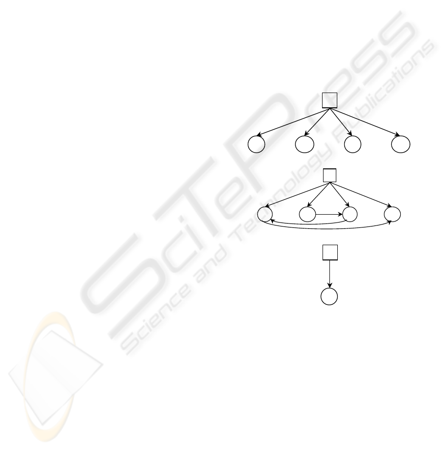
a)
X
3
X
2
X
1
X
p
…
C
b)
X
3
X
2
X
1
X
4
C
c)
X
C
Figure 1: Different bayesian network classifiers: NBN (a),
TAN (b) and CSNBN (c).
4 MULTIVARIATE CONTROL
CHARTS MODELIZED WITH
BAYESIAN NETWORK
The purpose of this article is to present a method
allowing the fault detection in a multivariate pro-
cess with the use of a BN. In the section 2, we
have presented the multivariate control charts T
2
and
MEWMA. It can be remarked that for these two
charts, one needs to compute a statistical distance on
ICINCO 2007 - International Conference on Informatics in Control, Automation and Robotics
230

the form of X
T
Σ
−1
X which is known as the square
Mahalanobis distance. This distance is also used in a
Discriminant Analysis (DA).
Indeed, one can distinguish two aspects of dis-
criminant analysis: the predictive and the classifica-
tion aspect. Given a system with p variables (descrip-
tors) and with k identified classes, the predictive dis-
criminant analysis (or Fisher discriminant analysis) is
generally used to find k − 1 new descriptors of a sys-
tem. These new k − 1 descriptors (which are a lin-
ear combination of the original descriptors) are sup-
posed to maximally discriminate between the k iden-
tified classes of the system. The other aspect of the
discriminant analysis is the classification one. The
purpose of the classification is principally to allocate
a new observation to one of the k identified classes of
the system. In the remainder of the article, the Dis-
criminant Analysis (DA) will be viewed only as a su-
pervised classification method (Duda et al., 2001).
DA is based on the Bayes decision rule. This rule
allocates a new observation x to the class C
i
with the
maximum a posteriori probability p(C
i
|x) giving the
value of each descriptor, as defined in the equation 5.
x ∈ C
i
, if i = argmax
i=1,...,k
{p(C
i
|x)} (5)
This decision rule is named ”Bayes decision rule”
because it is based on the Bayes rule which gives the
value of p(C
i
|x) as stated in 6.
P(C
i
|x) =
p(C
i
)p(x|C
i
)
p(x)
(6)
where p(C
i
) is the marginal probability of belong-
ing to the class C
i
. We can see that for each class,
the denominator of the equation 6 is the same, so, it
is not implicated in the discriminant function. Then,
equation 5 can be rewritten as:
x ∈ C
i
, if i = argmax
i=1,...,k
{p(C
i
)p(x|C
i
)} (7)
In industrial systems, it is usual to assume that
data follow multivariate normal distribution. The den-
sity function conditionally to a class C
i
can be written
as in equation 8, where µ
i
is the mean vector of the
class C
i
, Σ
i
is the covariance matrix of the class C
i
and |Σ
i
| represents the determinant of the matrix Σ
i
.
φ(x|C
i
) =
exp(−
1
2
(x− µ
i
)
t
Σ
−1
i
(x− µ
i
))
(2π)
p/2
|Σ
i
|
1/2
(8)
We remind that, for n samples, the Maximum
Likelihood Estimation (MLE) gives (Duda et al.,
2001):
ˆµ =
1
n
n
∑
i=1
x
i
(9)
and:
ˆ
Σ =
1
n− 1
n
∑
i=1
(x
i
− ˆµ)(x
i
− ˆµ)
t
(10)
So, if our system has k classes, the different prob-
abilities can be computed with equation 11.
p(x|C
i
) =
φ(x|C
i
)
k
∑
j=1
p(C
j
)φ(x|C
j
)
(11)
So, the equation 7 can be rewritten by the equation
12.
x ∈ C
i
, if i = argmax
i=1,...,k
p(C
i
)φ(x|C
i
)
k
∑
j=1
φ(x|C
j
)
(12)
At the first view, we can tell that the DA is well
suited for the fault diagnosis of industrial systems.
But, we will show that we can also realize the fault
detection methods of the multivariate control charts
with a DA, and particularly with a BN. So, to do that
we will consider the multivariate control charts as a
DA where the goal is to attribute a class (in or out of
control) to a new observation of the system. Realising
a DA with a BN is very simple. The structure of the
network will be composed of a class node (discrete
variable) with two modalities (in or out of control). In
order to represent the different descriptors of the sys-
tem, we use only one normal multivariate variable.
This normal multivariate variable will represent the x
for the T
2
chart and the y
t
for the MEWMA chart.
To resume, we will obtain a structure similar to the
CSNBN.
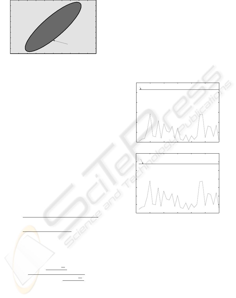
However, an essential question we remain con-
cerning the parameters of the network. We have to
fix a normal multivariate distribution for each classes
of the problem. The distribution of the ”in control”
state will be N(µ, Σ). In order to obtain a decision
boundary between the two states of the process, we
fix the distribution of the ”out of control” state to
N(µ,c × Σ), where c is a coefficient different than 1.
These two distributions will have same center (µ) and
same shape (because c× Σ is simply a scale extend-
ing of the shape of Σ). The difference between the two
states can be expressed as: scattering about the ”out
of control” state (OC) is more important than scatter-
ing about the ”in control” state (IC). We can represent
MULTIVARIATE CONTROL CHARTS WITH A BAYESIAN NETWORK
231
−5 −4 −3 −2 −1 0 1 2 3 4 5
−5
−4
−3
−2
−1
0
1
2
3
4
5
Out of Control
"OC"
In Control
"IC"
Control Limit
Figure 2: Example of the classification areas.
the classification areas of the two states of the system
for a bivariate example like in the figure 2.
Usually, in the frame of Statistical Process Con-
trol (SPC) techniques, one has to choose a risk factor
α in order to correctly control the process. In the case
of the BN, we have to fix a probability threshold τ al-
lowing to not badly reject some situations ”in control”
(false alarms).
Otherwise the threshold τ is computed in order to
have similar classification areas than those of the mul-
tivariate control chart. We will name CL the control
limit for the control charts and we supposed that CL is
known for each chart, see (Montgomery, 1997; Lowry
et al., 1992). The τ probability limit corresponds to
the probability, for the class ”OC”, of the x
CL
value
which is an observation giving a T
2
equal at the con-
trol limit CL. We will assume that the marginal prob-
abilities of the two classes are unknown and so are
fixed to 0.5 each. So, p(IC) = p(OC) = 0.5.
τ = p(IC|x
CL
)
=
p(OC)φ(x
CL
|OC)
p(IC)φ(x
CL
|IC) + p(OC)φ(x
CL
|OC)
=
φ(x
CL
|OC)
φ(x
CL
|IC) + φ(x
CL
|OC)
(13)
By using equation 8 in the previous equation, and
after simplification, we will obtain the equation of τ
as:
τ =
exp(−0.5
CL
c
)
c
p/2
exp(−0.5CL) +
exp(−0.5
CL
c
)
c
p/2
(14)
In conclusion, for the BN, we will obtain the fol-
lowing decision rule: if p(OC|x) ≥ τ, then the pro-
cess is out-of-control (OC), otherwise the process is
in control (IC).
In order to use the previous result, we have taken
a simple example of a 5 variables system. The param-
eters of the system is given as:
µ = [510]
Σ =
1 1.2
1.2 2
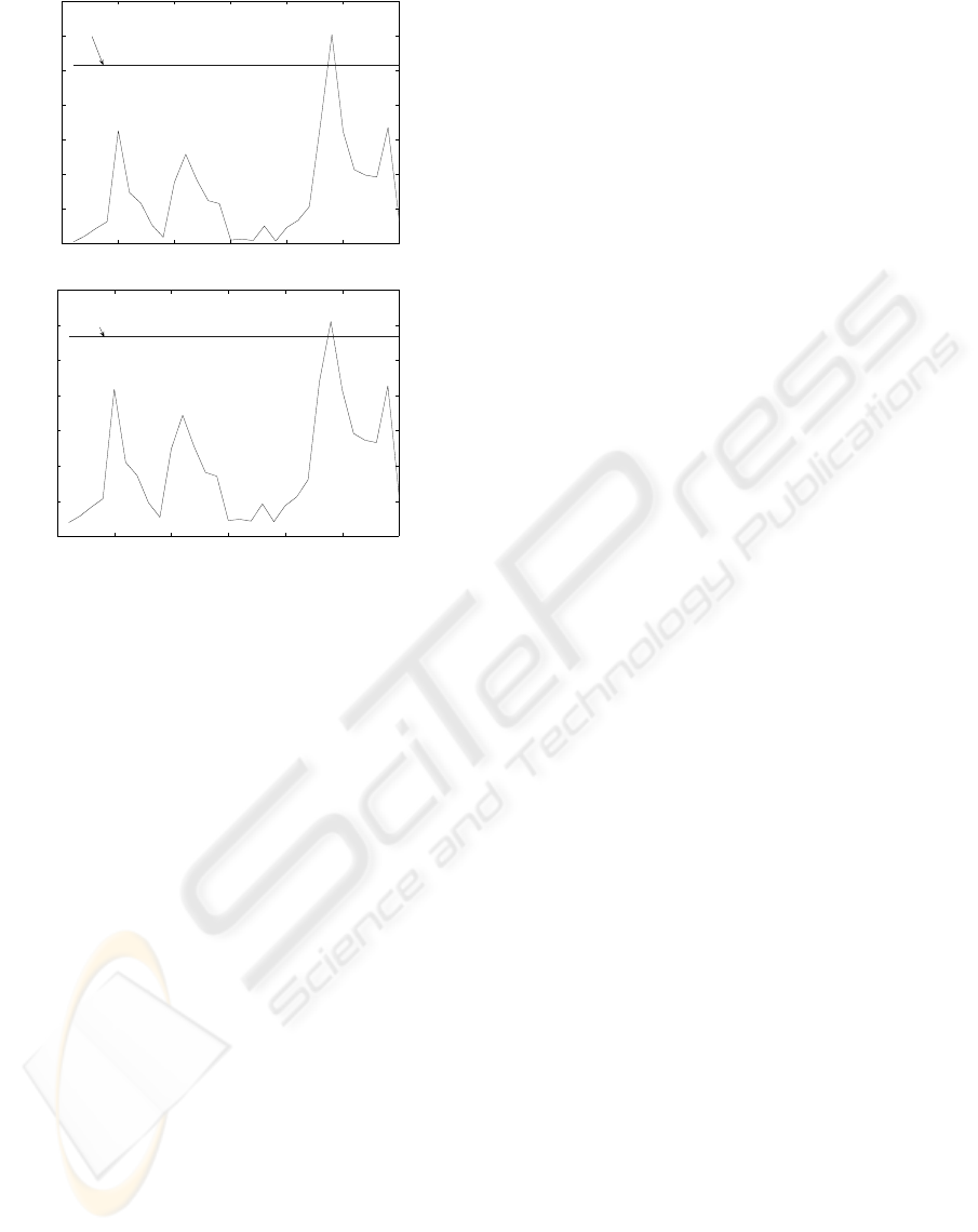
We have simulated the system during 30 observa-
tions, but at the observation number 6, a step of mag-
nitude 0.5 is introduced in the process. In the figure
3 we are presenting the detection of the fault with the
control chart (upper graph) and with the BN approach
(lower graph). In a similar way, the figure 4 represents
the result of the MEWMA approach.
0 5 10 15 20 25 30
0
2
4
6
8
10
12
Observations
T
2
CL
T
2
0 5 10 15 20 25 30
0.4
0.5
0.6
0.7
0.8
0.9
1
Observations
p(OC|x)
τ
Figure 3: Results with the T
2
chart and the T
2
chart by BN
apporach.
On the figure 3 and 4, we can see that for each
multivariate charts, the BN approach gives the same
results than the specified chart (with a scaling factor).
So, we can conclude that the different multivariate
control charts (T
2
and MEWMA) can be easily mod-
eled with a BN.
5 CONCLUSIONS AND
OUTLOOKS
In this article, after an introduction on the process
control (and particularly on the data-driven tech-
niques for the detection and the diagnosis), we have
ICINCO 2007 - International Conference on Informatics in Control, Automation and Robotics
232
0 5 10 15 20 25 30
0
2
4
6
8
10
12
14
Observations
T
2
mewma
CL
mewma
0 5 10 15 20 25 30
0.4
0.5
0.6
0.7
0.8
0.9
1
Observations
p(OC|y)
τ
mewma
Figure 4: Results with the MEWMA chart and the
MEWMA chart by BN approach.
outlined the problem that there is not a single tool able
to perform both: the fault detection and the fault di-
agnosis of a system. As a bayesian network can be an
efficient way to diagnosis a fault, it is natural to see
how this tool can also execute the fault detection task.
We have selected two fault detection techniques: the
T
2
chart and the MEWMA chart. We have demon-
strated that these charts can be viewed as a discrimi-
nant analysis and so can be implemented in a simple
bayesian network.
The evident outlook to this work is the full study
of the use of BN in order to monitor and control a
multivariate process.
REFERENCES
Bakshi, B. R. (1998). Multiscale PCA with application
to multivariate statistical process monitoring. AIChE
Journal, 44(7):1596–1610.
Bodden, K. and Rigdon, S. (1999). A program for approxi-
mating the in-control arl for the mewma chart. Journal
of Quality Technology, 31(1):120–123.
Chiang, L. H., Russell, E. L., and Braatz, R. D. (2001).
Fault detection and diagnosis in industrial systems.
New York: Springer-Verlag.
Cover, T. and Hart, P. (1967). Nearest neighbor pattern clas-
sification. IEEE Transactions on Information Theory,
13:21–27.
Duda, R. O., Hart, P. E., and Stork, D. G. (2001). Pattern
Classification 2nd edition. Wiley.
Friedman, N., Geiger, D., and Goldszmidt, M. (1997).
Bayesian network classifiers. Machine Learning,
29(2-3):131–163.
Hotelling, H. (1947). Multivariate quality control. Tech-
niques of Statistical Analysis, :111–184.
Jackson, E. J. (1985). Multivariate quality control. Com-
munication Statistics - Theory and Methods, 14:2657
– 2688.
Jensen, F. V. (1996). An introduction to Bayesian Networks.
Taylor and Francis, London, United Kingdom.
Kano, M., Nagao, K., Hasebe, S., Hashimoto, I., Ohno,
H., Strauss, R., and Bakshi, B. (2002). Comparison
of multivariate statistical process monitoring methods
with applications to the eastman challenge problem.
Computers and Chemical Engineering, 26(2):161–
174.
Kononenko, I. (1991). Semi-naive bayesian classifier. In
EWSL-91: Proceedings of the European working ses-
sion on learning on Machine learning, pages 206–
219.
Kourti, T. and MacGregor, J. F. (1996). Multivariate spc
methods for process and product monitoring. Journal
of Quality Technology, 28(4):409–428.
Langley, P., Iba, W., and Thompson, K. (1992). An analy-
sis of bayesian classifiers. In National Conference on
Artificial Intelligence.
Lowry, C. A., Woodall, W. H., Champ, C. W., and Rig-
don, S. E. (1992). A multivariate exponentially
weighted moving average control chart. Technomet-
rics, 34(1):46–53.
MacGregor, J. and Kourti, T. (1995). Statistical process
control of multivariate processes. Control Engineer-
ing Practice, 3(3):403–414.
Montgomery, D. C. (1997). Introduction to Statistical Qual-
ity Control, Third Edition. John Wiley and Sons.
Pearl, J. (1988). Probabilistic Reasoning in Intelligent Sys-
tems: Networks of Plausible Inference. Morgan Kauf-
mann Publishers.
Perez, A., Larranaga, P., and Inza, I. (2006). Super-
vised classification with conditional gaussian net-
works: Increasing the structure complexity from naive
bayes. International Journal of Approximate Reason-
ing, 43:1–25.
Pignatiello, J. and Runger, G. (1990). Comparisons of mul-
tivariate cusum charts. Journal of Quality Technology,
22(3):173–186.
Shewhart, W. A. (1931). Economic control of quality of
manufactured product. New York : D. Van Nostrand
Co.
Vapnik, V. N. (1995). The Nature of Statistical Learning
Theory. Springer.
MULTIVARIATE CONTROL CHARTS WITH A BAYESIAN NETWORK
233
