EVOLUTIONARY PATH PLANNING FOR UNMANNED AERIAL
VEHICLES COOPERATION
Ioannis K. Nikolos and Nikos Tsourveloudis
Intelligent Systems and RoboticsLaboratory, Technical University of Crete, Chania, Greece
Keywords: 3-D Path Planning, Evolutionary Algorithms, Navigation
, UAV cooperation, B-Splines.
Abstract: We suggest an evolutionary based off-line/on-line path planner for cooperating Unmanned Aerial Vehicles
(UAVs) that takes into account the environment characteristics and the flight envelope and mission
constraints of the cooperating UAVs. The scenario under consideration is the following: a number of UAVs
are launched from the same or different known initial locations. The main issue is to produce 3-D
trajectories that ensure a collision free operation with respect to mission constraints. The path planner
produces curved routes that are represented by 3-D B-Spline curves. Two types of planner are discussed:
The off-line planner generates collision free paths in environments with known characteristics and flight
restrictions. The on-line planner, which is based on the off-line one, generates collision free paths in
unknown static environments, by using acquired information from the UAV’s on-board sensors. This
information is exchanged between the cooperating UAVs in order to maximize the knowledge of the
environment. Both off-line and on-line path planning problems are formulated as optimization problems,
with a Differential Evolution algorithm to serve as the optimizer.
1 INTRODUCTION
Path planning is the generation of a space path
between an initial location and the desired
destination that has an optimal or near-optimal
performance under specific constraints (Gilmore,
1991). Searching for optimal paths is not a trivial
task; in most cases results in excessive computation
time and in some cases even the computation of just
a feasible path is a very difficult problem. Therefore,
in most cases we search for suboptimal or just
feasible solutions.
Unmanned Aerial Vehicles (UAVs) path planning
alg
orithms were initially developed for the solution
of the single vehicle case. However, the
continuously increasing interest for cooperating
UAVs resulted in the development of algorithms that
take into account the special issues and
characteristics of such missions. Cooperation
between UAVs has gained recently an increased
interest as systems of multiple vehicles engaged in
cooperative behavior show specific benefits
compared to a single vehicle. Cooperative behavior
may be defined as follows (Cao et al., 1999): Given
some tasks specified by a designer, a multiple robot
system displays cooperative behavior if, due to some
underlying mechanism, i.e. the “mechanism of
cooperation”, there is an increase in the total utility
of the system.
Path planning problems are computationally
d
emanding multi-objective multi-constraint
optimization problems (Mettler et al., 2003). The
problem complexity increases when multiple UAVs
should be used. Various approaches have been
reported for UAVs coordinated route planning, such
as Voronoi diagrams (Beard et al., 2002), mixed
integer linear programming (Richards et al., 2002),
(Schouwenaars et al., 2004) and dynamic
programming formulations (Flint et al., 2002).
Computational intelligence methods, such as Neural
Networks (Ortega and Camacho, 1996), Fuzzy
Logic (Kwon and Lee, 2000) and Evolutionary
Algorithms (EAs), (Nikolos et al., 2003), (Zheng et
al., 2005) have been successfully used to produce
trajectories for guiding mobile robots in known,
unknown or partially known environments.
EAs have been successfully used in the past for
t
he solution of the path-finding problem in ground
based or sea surface navigation (Michalewicz,
1999). A common practice was to model the path
67
K. Nikolos I. and Tsourveloudis N. (2007).
EVOLUTIONARY PATH PLANNING FOR UNMANNED AERIAL VEHICLES COOPERATION.
In Proceedings of the Fourth International Conference on Informatics in Control, Automation and Robotics, pages 67-75
DOI: 10.5220/0001642200670075
Copyright
c
 SciTePress

using straight line segments, connecting successive
way points. In the case of partially known or
dynamic environments a feasible and safe trajectory
was planned off-line by the EA and the algorithm
was used on-line whenever unexpected obstacles
were sensed (Smierzchalski, 1999), (Smierzchalski
and Michalewicz, 2000). EAs have been also used
for solving the path-finding problem in a 3-D
environment for underwater vehicles, assuming that
the path is a sequence of cells in a 3-D grid
(Sugihara and Yuh, 1997).
In (Nikolos et al., 2003) an EA based framework
was utilized to design an off-line / on-line path
planner for UAVs, which calculates a curved path
line represented by B-Spline curves in a 3-D
environment. The coordinates of the B-Spline
control points serve as design variables. For both
off-line and on-line planners, the problem is
formulated as an optimization one. Constraints are
formulated using penalty functions.
The work in this paper is the outgrowth of the one
presented in (Nikolos et al., 2003) for the case of
multiple and cooperating UAVs. The scenario
considered here is the following: a number of UAVs
are launched from the same or different known
initial locations with predefined initial directions.
The main issue is to produce 3-D trajectories,
represented by 3-D B-Spline curves, which connect
the initial locations with a single destination location
and ensure a collision free operation with respect to
mission constraints.
Two types of path planner are discussed: The off-
line planner generates collision free paths in
environments with known characteristics and flight
restrictions. The on-line planner, being an extension
of the off-line one and based on the ideas presented
in (Nikolos et al., 2003) was developed to generate
collision free paths in unknown environments. The
knowledge of the environment is gradually acquired
through the on-board sensors that scan the area
within a certain range from each UAV. This
information is exchanged between the cooperating
UAVs in order to maximize the sensors
effectiveness. The on-line planner rapidly generates
a near optimum path for each vehicle that will guide
the vehicle safely to an intermediate position within
the known territory, taking into account the mission
and cooperation objectives and constraints. The
process is repeated until the corresponding final
position is reached by an UAV. Then, each one of
the remaining UAVs uses the acquired information
about the environment and the off-line planner
output to compute a path that connects its current
position and the final destination. Both path
planning problems are formulated as optimization
(minimization) problems, where specially
constructed functions take into account mission and
cooperation objectives and constraints, with a
differential evolution algorithm to serve as the
optimizer.
The rest of the chapter is organized as follows:
section 2 contains B-Spline and differential
evolution algorithms fundamentals. The off-line path
planner will be briefly discussed in section 3.
Section 4 deals with the concept of cooperating
UAV on-line path planning using differential
evolution. The problem formulation is described,
including assumptions, objectives, constraints, cost
function definition and path modeling. Simulations
results are presented in section 5, followed by
discussion and conclusions in section 6.
2 DIFFERENTIAL EVOLUTION
OF B-SPLINE PATHS
2.1 Path Modelling using B-Splines
Straight-line segments that connect a number of
waypoints have been used in the past to model UAV
paths in 2D or 3D space (Moitra, 2003), (Zheng et
al., 2005). However, these simplified paths cannot
be used for an accurate simulation of UAV’s flight,
unless a large number of waypoints is adopted.
Furthermore, if an optimization procedure is used,
the number of design variables explodes, especially
if cooperating flying vehicles are considered. As a
result, the computation time becomes impractical for
real world applications.
B-Spline curves have been used in the past for
trajectory representation in 2-D (Alfaro and Garcia,
1988) or in 3-D environments (Nikolos et al., 2003),
(Nikolos et al., 2001). Their parametric construction
provides the ability to produce non-monotonic
curves, like the trajectories of moving objects. If the
number of control points of the corresponding curve
is n+1, with coordinates (x
0
, y
0
, z
0
) ,…, (x
n
, y
n
, z
n
),
the coordinates of the B-Spline curve may be written
as:
() ()
,
0
n
iip
i
x
uxN
=
=⋅
∑
u
,
(1)
ICINCO 2007 - International Conference on Informatics in Control, Automation and Robotics
68

() ()
,
0
n
iip
i
y
uyN
=
=⋅
∑
u
n
,
,
(2)
() ()
,
0
n
iip
i
zu z N u
=
=⋅
∑
,
(3)
where u is the free parameter of the curve, N
i,p
(u) are
the blending functions of the curve and p is its
degree, which is associated with curve’s smoothness
(p+1 being its order). Higher values of p correspond
to smoother curves (Farin, 1988).
The blending functions are defined recursively in
terms of a knot vector U={u
0
,…, u
m
}, which is a
non-decreasing sequence of real numbers, with the
most common form being the uniform non-periodic
one, defined as:
01
1
1.
i
if i p
uipifpi
np if ni
<+
⎧
⎪
=− +≤≤
⎨
⎪
−+ <
⎩
(4)
The blending functions N
i,p
are computed using the
knot values defined above, as:
()
1
,0
1
0
ii
i
if u u u
Nu
otherwise
+
≤<
⎧
=
⎨
⎩
(5)
() () ()
1
,,1
11
.
ip
i
ip ip i p
ip i ip i
uu
uu
Nu N u N u
uu u u
++
−+
++++
−
−
=+
−−
1,1−
(6)
If the denominator of the two fractions in (6) is
zero, that fraction is defined to have zero value.
Parameter u varies between 0 and (n-p+1) with a
constant step, providing the discrete points of the B-
Spline curve. The sum of the values of the blending
functions for any value of u is always 1.
2.2 Differential Evolution Algorithm
Differential Evolution (DE) (Price et al., 2005) is
used in this work as the optimization tool. The
classic DE algorithm evolves a fixed size
population, which is randomly initialized. After
initializing the population, an iterative process is
started and at each generation , a new population
is produced until a stopping condition is satisfied. At
each generation, each element of the population can
be replaced with a new generated one. The new
element is a linear combination between a randomly
selected element and the difference between two
other randomly selected elements. Below, a more
analytical description of the algorithm’s structure is
presented.
G
Given a cost function ,
the optimization target is to minimize the value of
this cost function by optimizing the values of its
parameters (design variables), that is
()
:
param
n
fX →
(
)
12
,,, ,
param
nj
Xxx x x
=
∈…
,
(7)
where X denotes the vector composed of n
param
cost
function parameters (design variables). These
parameters take values between specific upper and
lower bounds, as follows:
(
)
(
)
,1,,
LU
j
jj para
xxxj n≤≤ =…
m
(8)
The DE algorithm implements real encoding for
the values of the objective function’s variables. In
order to obtain a starting point for the algorithm, an
initialization of the population takes place. The
initialization (for
1G
=
) is established by randomly
assigning values to the parameters of each
member of the population, within the given
boundaries
j
i
() ( ) ( )
(
)
()
1
,
, 1,, , 1,,
UL L
i j j j j pop param
xrx x xi n j n=⋅ − + = =……
(9)
where r is a uniformly distributed random value
within range [0, 1]. DE’s mutation operator is based
on a triplet of randomly selected different
individuals. For each
i
member of the population, a
new parameter vector V
i
(G)
is generated by adding
the weighted difference vector between the two
members of the triplet to the third one (the donor).
That is:
() () () ()
(
)
() () () ()
(
)
31
,1 , 2
,
,
,,, ,
ii
param
GG GG
i
rrr
GGG G
i
ii
in
VXFXX
Vvvv
=+⋅ −
= …
2
i
(10)
where
(
)
3
i
G
r
X is called the “donor”, G is the current
generation, and
[][]
1, , , 1, ,
11,, ,21,, ,31,,
123
0,1 , 0,1
pop param
i pop i pop i pop
iii
injn
rnr nr n
rr ri
Fr
=
=
⎡
⎤⎡ ⎤⎡
∈∈∈
⎤
⎣
⎦⎣ ⎦⎣
≠≠≠
∈+∈
……
………
⎦
(11)
In this way a perturbed individual is generated.
The perturbed individual V
i
(G)
and the initial
population member X
i
(G)
are then subjected to a
crossover operation that generates the final
candidate solution
(
)
1G
i
U
+
EVOLUTIONARY PATH PLANNING FOR UNMANNED AERIAL VEHICLES COOPERATION
69

()
()
()
()
[]
,
1
,
,
1, ,
0,1
G
i j r param
G
ij
G
ij
r
vifrCjkj n
u
xotherwise
C
+
⎧
≤∨=∀=
⎪
=
⎨
⎪
⎩
∈
…
(12)
where k is a random integer within [1, n
param
],
chosen once for all members of the population. The
random number is seeded for every gene of each
chromosome. F and C
r
r
are DE control parameters,
which remain constant during the search process and
affect the convergence behaviour and robustness of
the algorithm. Their values also depend on the
objective function, the characteristics of the problem
and the population size.
The population for the next generation (G+1) is
selected between the current population and the final
candidates. If each candidate vector is better fitted
than the corresponding current one, the new vector
replaces the vector with which it was compared. The
DE selection scheme is described as follows (for a
minimization problem):
()
() ()
(
)
()
(
)
()
11
1
GG
ii
G
i
G
i
UiffU fX
X
Xotherwise
++
+
⎧
≤
⎪
=
⎨
⎪
⎩
G
i
(13)
Α new scheme (Hui-Yuan et al., 2003) to
determine the donor for mutation operation has been
adopted for accelerating the convergence rate. In this
scheme, donor is randomly selected (with uniform
distribution) from the region within the “hyper-
triangle”, formed by the three members of the triplet
presented below:
() ()
[]
33
11
01
i
GG
ikmm
rk
km
donor λλX,λ rand ,
==
⎛⎞
=
⎜⎟
⎜⎟
⎝⎠
∑∑
=
(14)
where rand [0, 1] denotes a uniformly distributed
value within the range [0, 1]. With this scheme the
donor comprises the local information of all
members of the triplet, providing a better starting-
point for the mutation operation that result in a better
distribution of the trial-vectors.
The random number generation (with uniform
probability) is based on the algorithm presented in
(Marse and Roberts, 1983). In each different
operation inside the DE algorithm that requires a
random number generation, a different sequence of
random numbers is produced, by using a different
initial seed for each operation and a separate storage
of the corresponding produced seeds.
3 OFF-LINE PATH PLANNER
The off-line planner generates collision free paths in
environments with known characteristics and flight
restrictions. The derived path lines are continuous 3-
D B-Spline curves.
Each B-Spline control point is defined by its
three Cartesian coordinates x
k,j
, y
k,j
, z
k,j
(k=0,…,n,
j=1,…,N), N is the number of UAVs, while n+1 is
the number of control points in each B-Spline curve
(the same for all curves). The first (k=0) and last
(k=n) control points of the control polygon are the
initial and target points of the j
th
UAV, which are
predefined by the user. The second (k=1) control
point is positioned in a pre-specified distance from
the first one, in a given altitude, and in a given
direction, in order to define the initial direction of
the corresponding path.
For the case of a single UAV the optimization
problem to be solved minimizes a set of five terms,
connected to various objectives and constraints; they
are associated with the feasibility of the curve, its
length and a safety distance from the ground. The
cost function to be minimized is defined as:
5
1
ii
i
f
wf
=
=
∑
(15)
Term f
1
penalizes the non-feasible curves that
pass through the solid boundary. In order to compute
this term, discrete points along each curve are
computed, using B-Spline equations (Eq. 1 to 6) and
a pre-specified step for B-Spline parameter u.
Term f
2
is the length of the curve (non-
dimensional with the distance between the starting
and destination points) and is used to provide shorter
paths.
Term f
3
is designed to provide flight paths with a
safety distance from solid boundaries.
Term f
4
is designed to provide B-Spline curves
with control points inside the pre-specified space.
Term f
5
was designed to provide path lines within
the known terrain. This characteristic is particularly
useful when the off-line path planner is used
together with the on-line one, as it will be explained
later.
Weights w
i
are experimentally determined, using
as criterion the almost uniform effect of the last four
terms in the objective function. Term w
1
f
1
has a
dominant role in (15) providing feasible curves in
few generations, since path feasibility is the main
concern. The minimization of (15), through the DE
procedure, results in a set of B-Spline control points,
which actually represents the desired path.
ICINCO 2007 - International Conference on Informatics in Control, Automation and Robotics
70

4 ON-LINE PATH PLANNING
Having N UAVs launched from the same or
different known initial locations, the issue is to
produce N 3-D trajectories, aiming at reaching a
predetermined target location, while ensuring
collision avoidance with the environmental
obstacles. Additionally, the produced flight paths
should satisfy specific route constraints. Each
vehicle is assumed to be a point, while its actual size
is taken into account by equivalent obstacle –
ground growing.
The general constraint of the problem is the
collision avoidance between UAVs and the ground.
The route constraints are:
(a) Predefined initial and target coordinates for
all UAVs
(b) Predefined initial directions for all UAVs,
(c) Predefined minimum and maximum limits of
allowed-to-fly space (minimum and maximum
allowed Cartesian coordinates for all path points).
The cooperation objective is that all UAVs
should reach the same target point.
The on-line planner uses acquired information
from all UAV’s on-board sensors (that scan the area
within a certain range from the corresponding
UAV). The planner rapidly generates a near
optimum path, modeled as a 3-D B-Spline curve that
will guide each vehicle safely to an intermediate
position within the already scanned area. The
information about the already scanned area by each
UAV is passed to the rest cooperating UAVs, in
order to maximize the knowledge of the
environment. The process is repeated until the final
position is reached by a UAV. Then the rest of
UAVs turn to the off-line mode and a single B-
Spline path for each UAV is computed to guide the
corresponding vehicle from its current position,
through the already scanned territory to the common
final destination. As a result, each path line from the
corresponding starting point to the final goal is a
smooth, continuous 3-D line that consists of
successive B-Spline curves, smoothly connected to
each other (Figure 1).
As the terrain is completely unknown and the
radars (or equivalent sensors) gradually scan the
area, it is impossible to generate feasible paths that
connect each starting point with the target one.
Instead, at certain moments, each sensor scans a
region around the corresponding moving UAV and
this region is added to the already scanned regions
by all cooperating UAVs. For the UAV under
consideration a path line is generated that connects a
temporary starting point with a temporary ending
point. Each temporary ending point is also the next
curve’s starting point for the corresponding vehicle.
Therefore, what is finally generated is a group of
smooth curve segments connected to each other,
eventually connecting the starting point to the final
destination for each UAV.
In the on-line problem only four control points
define each B-Spline curve, the first two of which
are fixed and determine the direction of the current
UAV path. The remaining two control points are
allowed to take any position within the scanned by
the radars known space, taking into consideration
given constraints.
When the next path segment is to be generated,
only the first control point of the B-Spline curve is
known (it is the last control point of the previous B-
Spline segment). The second control point is not
random as it is used to make sure that at least first
derivative continuity of the two connected curves is
provided at their common point. Hence, the second
control point of the next curve should lie on the line
defined by the last two control points of the previous
curve.
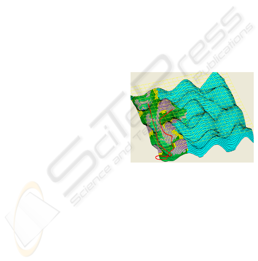
Figure 1: On-line path planning for a single UAV. The
path is shown in an intermediate position of the UAV’s
flight. The already scanned area is presented in color.
The path-planning algorithm considers the
scanned surface as a group of quadratic mesh nodes.
All ground nodes are initially considered unknown.
Radar information is used to produce the first path
line segment for the corresponding UAV. As the
vehicle is moving along its first segment and until it
has travelled about 2/3 of its length, its radar scans
the surrounding area, returning a new set of visible
nodes, which are subsequently added to the common
set of scanned nodes. The on-line planner, then,
produces a new segment for each UAV, whose first
point is the last point of the previous segment and
whose last point lies somewhere in the already
scanned area, its position being determined by the
on-line procedure. The on-line process is repeated
until the ending point of the current path line
EVOLUTIONARY PATH PLANNING FOR UNMANNED AERIAL VEHICLES COOPERATION
71

segment of one UAV lies close to the final
destination. Then the rest UAVs turn into the off-
line process, in order to reach the target using B-
Spline curves that pass through the scanned terrain.
The computation of intermediate path segments
for each UAV is formulated as a minimization
problem. The cost function to be minimized is
formulated as the weighted sum of eight different
terms:
8
1
ii
i
f
wf
=
=
∑
,
(16)
where w
i
are the weights and f
i
are the corresponding
terms described below.
Terms f
1
, f
2
, and f
3
are the same with terms f
1
, f
3
,
and f
4
respectively of the off-line procedure. Term f
1
penalizes the non-feasible curves that pass through
the solid boundary. Term f
2
is designed to provide
flight paths with a safety distance from solid
boundaries. Only already scanned ground points are
considered for this calculation. Term f
3
is designed
to provide B-Spline curves with control points inside
the pre-specified working space.
Term f
4
is designed to provide flight segments
with their last control point having a safety distance
from solid boundaries. This term was introduced to
ensure that the next path segment that is going to be
computed will not start very close to a solid
boundary (which may lead to infeasible paths or
paths with abrupt turns). The minimum distance D
min
from the ground is calculated for the last control
point of the current path segment. Only already
scanned ground points are considered for this
calculation. Term f
4
is defined as:
()
2
4msafe
fdD=
in
,
(17)
where d
safe
represents a safety distance from the
solid boundary.
The value of term f
5
depends on the potential
field strength between the initial point of the UAVs
path and the final target. This potential field between
the two points is the main driving force for the
gradual development of each path line in the on-line
procedure. The potential is similar to the one
between a source and a sink, defined as:
01
02
ln
rcr
rcr
Φ
⋅+
⋅+
=
,
(18)
where r
1
is the distance between the last point of the
current curve and the initial point for the
corresponding UAV, r
2
is the distance between the
last point of the current curve and the final
destination, r
0
is the distance between the initial
point for the corresponding UAV and the final
destination and c is a constant.
This potential allows
for selecting curved paths that bypass obstacles lying
between the starting and ending point of each B-
Spline curve (Nikolos et al., 2003).
Term f
6
is similar to term f
5
but it corresponds to
a potential field between the current starting point
(of the corresponding path segment) and the final
target.
Term f
7
is designed to prevent UAVs from being
trapped in small regions and to force them move
towards unexplored areas. In order to help the UAV
leave this area, term f
7
repels it from the points of
the already computed path lines (of all UAVs).
Furthermore, if a UAV is wandering around to find a
path that will guide it to its target, the UAV will be
forced to move towards areas not visited before by
this or other UAVs. This term has the form:
7
1
11
po
N
po k
k
f
Nr
=
=
∑
,
(19)
where N
po
is the number of the discrete curve points
produced so far by all UAVs and r
k
is their distance
from the last point of the current curve segment.
Term f
8
represents another potential field, which
is developed in a small area around the final target.
When the UAV is away from the final target, the
term is given a constant value. When the UAV is
very close to the target the term’s value decreases
proportionally to the square of the distance between
the last point of the current curve and the target.
Weights w
i
in (16) are experimentally determined,
using as criterion the almost uniform effect of all the
terms, except the first one. Term w
1
f
1
has a dominant
role, in order to provide feasible curve segments in a
few generations, since path feasibility is the main
concern.
5 SIMULATION RESULTS
The same artificial environment was used for all test
cases considered here. The artificial environment is
constructed within a rectangle of 20x20 (non-
dimensional lengths). The (non-dimensional) radar’s
range for each UAV was set equal to 4. The safety
distance from the ground was set equal to d
safe
=0.25.
The (experimentally optimized) settings of the DE
algorithm during the on-line procedure were as
follows: population size = 20, F = 0.6, C
r
= 0.45,
number of generations = 70. For the on-line
procedure we have two free-to-move control points,
resulting in 6 design variables. The corresponding
ICINCO 2007 - International Conference on Informatics in Control, Automation and Robotics
72

settings during the off-line procedure were as
follows: population size = 30, F = 0.6, C
r
= 0.45,
number of generations = 70. For the off-line
procedure eight control points were used to construct
each B-Spline curve (including the initial (k=0) and
the final one (k=7). These correspond to five free-to-
move control points, resulting in 15 design variables.
All B-Spline curves have a degree p equal to 3. All
experiments have been designed in order to search
for path lines between “mountains”. For this reason,
an upper ceiling for flight height has been enforced
in the optimization procedure, by explicitly
providing an upper boundary for the z coordinates of
all B-Spline control points.
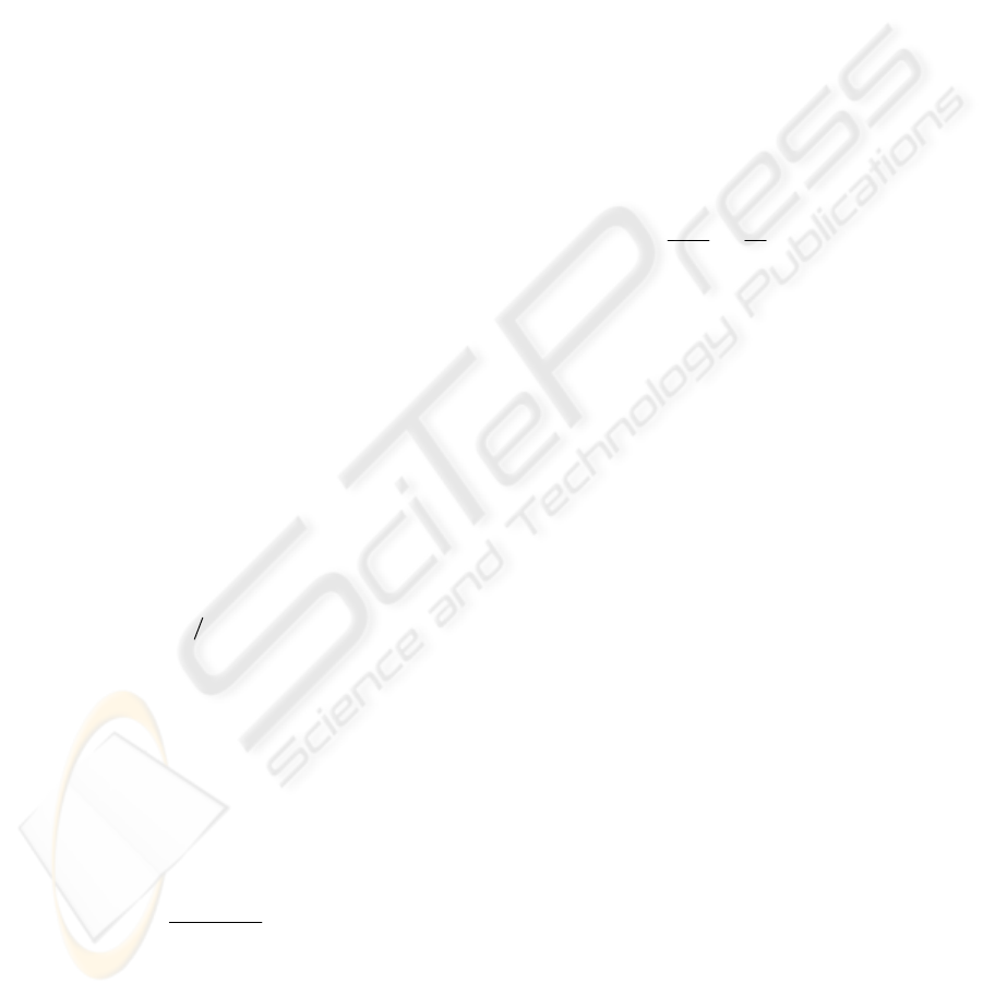
Figure 2: Test case 6 corresponds to the on-line path
planning of two UAVs. When the first UAV (blue line)
reaches the target the second one turns into the off-line
mode. The starting point for the first UAV is close to the
lower left corner of the terrain, while for the second one is
close to the upper left corner.
Test case 1 corresponds to on-line path planning
of two UAVs. Figure 2 shows the path lines when
the first UAV (blue line) reaches the target. In that
moment the second UAV (red line) turns into the
off-line mode, in order to compute a feasible path
line that connects its current position with the target,
through the already scanned area. The final status is
demonstrated in Figure 3. The starting point for the
first UAV is near the lower left corner of the terrain,
while for the second one is near the upper left
corner.
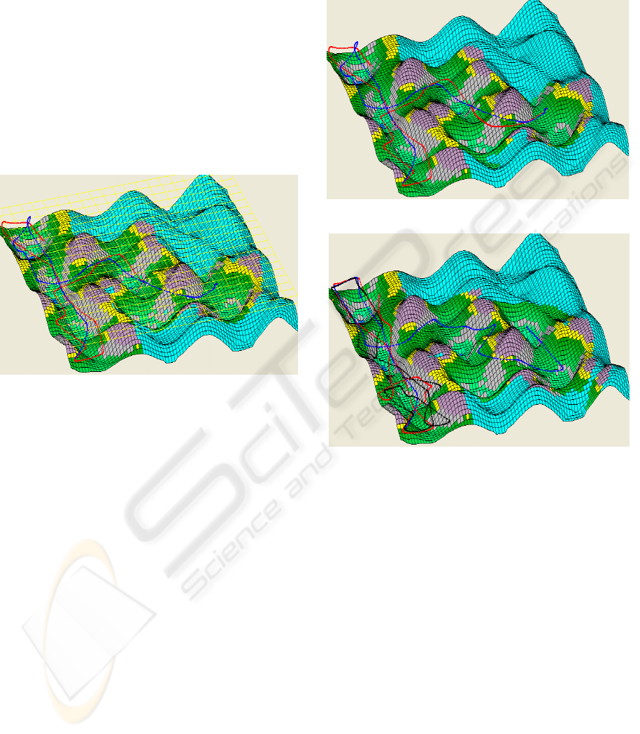
Test case 2 corresponds to the on-line path
planning of three UAVs. Figure 4 shows the status
of the two path lines when the first UAV (blue line)
reaches the target. In that moment the second UAV
(red line) and the third one (black line) turn into the
off-line mode, in order to compute feasible path
lines that connect their positions with the target. The
final paths for all three UAVs are demonstrated in
Figure 5. The starting point for the first and second
UAVs are the same as in case 1, while the third
UAV is near the middle of the left side of the terrain.
Figure 3: The final path lines for the test case 1.
Figure 4: On-line path planning of three cooperating
UAVs (test case 2). The picture shows the paths when the
first UAV (blue line) reaches the target.
Test case 3 also corresponds to the on-line path
planning of three UAVs but with distant starting
points. Figure 6 shows the status of the two path
lines when the first UAV (blue line) reaches the
target. The final status is demonstrated in Figure 7.
As the first UAV (blue line) is close to the target, it
succeeds in reaching it using just one B-Spline
segment. Then, the other two UAVs turn into off-
line mode to reach the target.
In the test case 4 three UAVs are launched from
the centre of the working space but towards different
directions. Figure 8 shows the status of the two path
lines when the first UAV (blue line) reaches the
target. The final status is demonstrated in Figure 9.
When the final point of a curve segment is within a
small distance from the final destination, the on-line
procedure is terminated; this is the reason for the
EVOLUTIONARY PATH PLANNING FOR UNMANNED AERIAL VEHICLES COOPERATION
73

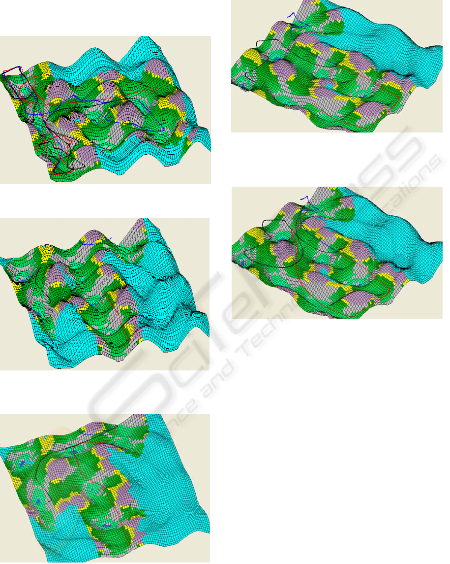
absence of coincidence between the final points of
the first (blue line) and the rest path lines.
Figure 5: The final paths of the test case 2.
Figure 6: Path lines of three distant UAVs when the first
one (blue line) reaches the target.
Figure 7: The final paths of test case 3.
Figure 8: On-line path planning for three UAVs launched
from the same point but different initial directions. The
first UAV (blue line) just reached the target.
Figure 9: The final paths of test case 4.
6 CONCLUSIONS
A path planner for a group of cooperating UAVs
was presented. The planner is capable of producing
smooth path curves in known or unknown static
environments. Two types of path planner were
presented. The off-line one generates collision free
paths in environments with known characteristics
and flight restrictions. The on-line planner, which is
based on the off-line one, generates collision free
paths in unknown environments. The path line is
gradually constructed by successive, smoothly
connected B-Spline curves, within the gradually
scanned environment. The knowledge of the
environment is acquired through the UAV’s on-
board sensors that scan the area within a certain
range from each UAV. This information is
exchanged between the cooperating UAVs; as a
result, each UAV utilizes the knowledge of a larger
region than the one scanned by its own sensors. The
on-line planner generates for each vehicle a smooth
ICINCO 2007 - International Conference on Informatics in Control, Automation and Robotics
74

path segment that will guide the vehicle safely to an
intermediate position within the known territory.
The process is repeated for all UAVs until the
corresponding final position is reached by an UAV.
Then, the rest vehicles turn into the off-line mode in
order to compute path lines consisting of a single B-
Spline curve that connect their current positions with
the final destination. These path lines are enforced to
lie within the already scanned region. Both path
planners are based on optimization procedures, and
specially constructed functions are used to encounter
the mission and cooperation objectives and
constraints. A differential evolution algorithm is
used as the optimizer for both planners. No
provision is taken by the on-line planner for
collision avoidance between the cooperating
vehicles; this can be encountered by an on board
controller for each vehicle.
REFERENCES
Gilmore, J.F., 1991. Autonomous vehicle planning
analysis methodology. In Proceedings of the
Association of Unmanned Vehicles Systems
Conference. Washington, DC, 503–509.
Zheng, C., Li, L., Xu, F., Sun, F., Ding, M., 2005.
Evolutionary Route Planner for Unmanned Air
Vehicles. IEEE Transactions on Robotics, 21, 609-
620.
Uny Cao, Y., Fukunaga, A.S., Kahng, A.B., 1997.
Cooperative Mobile Robotics: Antecedents and
Directions. Autonomous Robots, 4, 7-27.
Mettler, B., Schouwenaars, T., How, J., Paunicka, J., and
Feron E., 2003. Autonomous UAV guidance build-up:
Flight-test Demonstration and evaluation plan. In
Proceedings of the AIAA Guidance, Navigation, and
Control Conference, AIAA-2003-5744.
Beard, R.W., McLain, T.W., Goodrich, M.A., Anderson,
E.P., 2002. Coordinated target assignment and
intercept for unmanned air vehicles. IEEE
Transactions on Robotics and Automation, 18, 911-
922.
Richards, A., Bellingham, J., Tillerson, M., and How., J.,
2002. Coordination and control of UAVs. In
Proceedings of the AIAA Guidance, Navigation and
Control Conference, Monterey, CA.
Schouwenaars, T., How, J., and Feron, E., 2004.
Decentralized Cooperative Trajectory Planning of
multiple aircraft with hard safety guarantees. In
Proceedings of AIAA Guidance, Navigation, and
Control Conference and Exhibit, AIAA-2004-5141.
Flint, M., Polycarpou, M., and Fernandez-Gaucherand, E.,
2002. Cooperative Control for Multiple Autonomous
UAV’s Searching for Targets. In Proceedings of the
41st IEEE Conference on Decision and Control.
Gomez Ortega, J., and Camacho, E.F., 1996. Mobile
Robot navigation in a partially structured static
environment, using neural predictive control. Control
Eng. Practice, 4, 1669-1679.
Kwon, Y.D., and Lee, J.S., 2000. On-line evolutionary
optimization of fuzzy control system based on
decentralized population. Intelligent Automation and
Soft Computing, 6, 135-146.
Nikolos, I.K., Valavanis, K.P., Tsourveloudis, N.C.,
Kostaras, A., 2003. Evolutionary Algorithm based
offline / online path planner for UAV navigation.
IEEE Transactions on Systems, Man, and Cybernetics
– Part B: Cybernetics, 33, 898-912.
Michalewicz, Z., 1999. Genetic Algorithms + Data
Structures = Evolution Programs. Springer
Publications.
Smierzchalski, R., 1999. Evolutionary trajectory planning
of ships in navigation traffic areas. Journal of Marine
Science and Technology, 4, 1-6.
Smierzchalski, R., and Michalewicz Z., 2000. Modeling of
ship trajectory in collision situations by an
evolutionary algorithm. IEEE Transactions on
Evolutionary Computation, 4, 227-241.
Sugihara, K., and Yuh, J., 1997. GA-based motion
planning for underwater robotic vehicles. UUST-10,
Durham, NH.
Moitra, A., Mattheyses, R.M., Hoebel, L.J., Szczerba, R.J.,
Yamrom, B., 2003. Multivehicle reconnaissance route
and sensor planning. IEEE Transactions on Aerospace
and Electronic Systems, 37, 799-812.
Martinez-Alfaro H., and Gomez-Garcia, S. 1988. Mobile
robot path planning and tracking using simulated
annealing and fuzzy logic control. Expert Systems with
Applications, 15, 421-429.
Nikolos, I.K., Tsourveloudis, N., and Valavanis, K.P.,
2001. Evolutionary Algorithm Based 3-D Path Planner
for UAV Navigation. In Proceedings of the 9th
Mediterranean Conference on Control and
Automation, Dubrovnik, Croatia.
Farin, G., 1988. Curves and Surfaces for Computer Aided
Geometric Design, A Practical Guide. Academic
Press.
Price, K.V., Storn, R.M., Lampinen, J.A., 2005.
Differential Evolution, a Practical Approach to Global
Optimization. Springer-Verlag, Berlin Heidelberg.
Marse, K. and Roberts, S.D., 1983. Implementing a
portable FORTRAN uniform (0,1) generator.
Simulation, 41-135.
EVOLUTIONARY PATH PLANNING FOR UNMANNED AERIAL VEHICLES COOPERATION
75