ROBOT TCP POSITIONING WITH VISION

Accuracy Estimation of a Robot Visual Control System

Drago Torkar and Gregor Papa

Computer Systems Department, Jožef Stefan Institute, Jamova c. 39, SI-1000 Ljubljana, Slovenia

Keywords: Robot control, Calibrated visual servoing.

Abstract: Calibrated 3D visual servoing has not fully matured as a industrial technology yet, and in order to widen its

use in industrial applications its technological capability must be precisely known. Accuracy and

repeatability are two of the crucial parameters in planning of any robotic task. In this paper we describe a

procedure to evaluate the 2D and 3D accuracy of a robot stereo vision system consisting of two identical 1

Megapixel cameras, and present the results of the evaluation.

1 INTRODUCTION

In the last decades, more and more robots

applications were used in industrial manufacturing

which was accompanied by an increased demand for

versatility, robustness and precision. The demand

was mostly satisfied by increasing the mechanical

capabilities of robot parts. For instance, to meet the

micrometric positioning requirements, stiffness of

the robot’s arms was increased, high precision gears

and low backlash joints introduced, which often led

to difficult design compromises such as the request

to reduce inertia and increase stiffness. This results

in approaching the mechanical limits and increased

cost of robots decreasing the competitiveness of the

robot systems on the market (Arflex, 2005).

Lately, the robot producers have put much effort

into incorporating visual and other sensors to the

actual industrial robots thus providing a significant

improvement in accuracy, flexibility and

adaptability. Vision is still one of the most

promising sensors (Ruf and Horaud, 1999) in real

robotic 3D servoing issues (Hutchinson et al., 1995).

It has been vastly investigated for the last two

decades in laboratories but it's only now that it finds

its way to industrial implementation (Robson, 2006)

in contrast to machine vision which became a well

established industry in the last years (Zuech, 2000).

There are many reasons for this. The vision systems

used with the robots must satisfy a few constraints

that differ them from a machine vision measuring

systems. First of all, the camera working distances

are much larger, especially with larger robots that

can reach several meters. Measuring at such

distances with high precision requires much higher

resolution which very soon reaches its technological

and price limits. For example, nowadays 4

Megapixel cameras are the state of the art in vision

technology but are not affordable in many robotic

applications since their price almost reaches the

robot price. The dynamics of the industrial processes

requires high frame rates which in connection with

real time processing puts another difficult constraint

on system integrators. The unstructured industrial

environment with changing environmental lighting

is another challenge for the robot vision specialists.

When designing the vision system within robot

applications it is very important to choose the

optimal equipment for the task and to get maximal

performance out of each component. In the paper we

represent a procedure for the precision estimation of

a calibrated robot stereo vision system in 2D and 3D

environment. Such a system can be used in visual

servoing applications for precise tool center point

(TCP) positioning.

2 METHODOLOGY

Four types of accuracy tests were performed: a static

2D test, a dynamic 2D test, a static 3D test, and a

dynamic 3D test. Throughout all the tests, an array

of 10 infrared light emitting diodes (IR-LED) was

used to establish its suitability for being used as a

212

Torkar D. and Papa G. (2007).

ROBOT TCP POSITIONING WITH VISION - Accuracy Estimation of a Robot Visual Control System.

In Proceedings of the Fourth International Conference on Informatics in Control, Automation and Robotics, pages 212-215

DOI: 10.5220/0001643502120215

 SciTePress

marker and a calibration pattern in the robot visual

servoing applications.

Within the static 2D test, we were moving the

IR-LED array with the linear drive perpendicular to

the camera optical axes and measured the increments

in the image. The purpose was to detect the smallest

linear response in the image. The IR-LED centroids

were determined in two ways: on binary images and

on grey-level images as centers of mass. During

image grabbing the array did not move thus

eliminating any dynamic effects. We averaged the

movement of centroids of 10 IR-LEDs in a sequence

of 16 images and calculated the standard deviation

to obtain accuracy confidence intervals. With the

dynamic 2D test shape distorsions in the images due

to fast 2D movements of linear drive were

investigated. We compared a few images of IR-LED

array taken during movement to statically obtained

ones which provided information of photocenter

displacements and an estimation of dynamic error.

We performed the 3D accuracy evaluation with 2

fully calibrated cameras in a stereo setup. Using

again the linear drive, the array of IR-LEDs was

moved along the line in 3D space with different

increments and the smallest movement producing a

linear response in reconstructed 3D space was

sought. In the 3D dynamic test, we attached the IR-

LED array to the wrist of an industrial robot, and

dynamically guided it through some predefined

points in space and simultaneously recorded the

trajectory with fully calibrated stereo cameras. We

compared the reconstructed 3D points from images

to the predefined points fed to robot controller.

3 TESTING SETUP

The test environment consisted of:

 PhotonFocus MV-D1024-80-CL-8 camera with

CMOS sensor and framerate of 75 fps at full

resolution (1024x1024 pixels),

 Active Silicon Phoenix-DIG48 PCI frame

grabber,

 Moving object (IR-LED array) at approximate

distance of 2m. The IR-LED array (standard

deviation of IR-LED accuracy is below 0.007

pixel, as stated in (Papa and Torkar, 2006))

fixed to Festo linear guide (DGE-25-550-SP)

with repetition accuracy of +/-0.02mm.

For then static 2D test the distance from camera

to a moving object (in the middle position) that

moves perpendicularly to optical axis was 195cm;

camera field-of-view was 220cm, which gives pixel

size of 2.148mm; Schneider-Kreuznach lens

CINEGON 10mm/1,9F with IR filter; exposure time

was 10.73ms, while frame time was 24.04ms, both

obtained experimentally.

For the dynamic 2D test conditions were the

same as in static test, except the linear guide was

moving the IR-LED array with a speed of 460mm/s

and the exposure time was 1ms.

In the 3D reconstruction test the left camera

distance to IR-LED array and right camera distance

to IR-LED array were about 205cm; baseline

distance was 123cm; Schneider-Kreuznach lens

CINEGON 10mm/1,9F with IR filter; Calibration

region-of-interest (ROI): 342 x 333 pixels;

Calibration pattern: 6 x 8 black/white squares;

Calibration method (Zhang, 1998); Reconstruction

method (Faugeras, 1992). The reconstruction was

done off-line and the stereo correspondence problem

was considered solved due to a simple geometry of

the IR-LED array and is thus not addressed here.

For the 3D dynamic test, an ABB industrial robot

IRB 140 was used with the standalone fully

calibrated stereo vision setup placed about 2m away

from its base and calibrated the same way as before.

The robot wrist was moving through the corners of

an imaginary triangle with side length of

approximately 12cm. The images were taken

dynamically when the TCP was passing the corner

points and reconstructed in 3D with an approximate

speed of 500mm/s. The relative length of such

triangle sides were compared to the sides of a

statically-obtained and reconstructed triangle. The

robot native repeatability is 0.02 mm and its

accuracy is 0.01mm.

4 RESULTS

4.1 2D Accuracy Tests

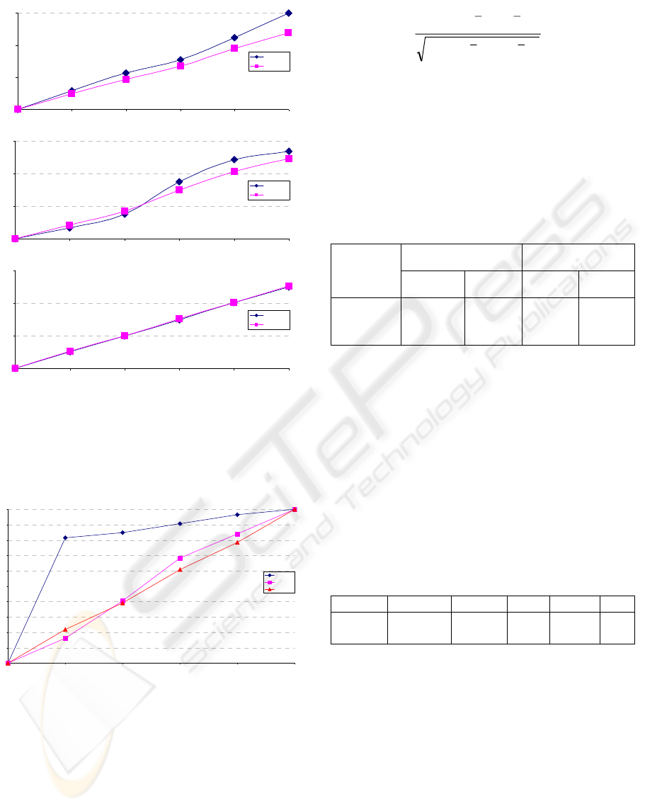
The results of the evaluation tests are given below.

Tests include the binary and grey-level centroids.

For each movement increment the two figures are

presented, as described below.

Pixel difference between the starting image and

the consecutive images (at consecutive positions) –

for each position the value is calculated as the

average displacement of all 10 markers, while their

position is calculated as the average position in the

sequence of the 16 images grabbed at each position

in static conditions. The lines in these figures should

be as straight as possible.

The 0.01mm, 0.1mm, and 1mm increments for

2D tests are presented in Figure 1.

ROBOT TCP POSITIONING WITH VISION - Accuracy Estimation of a Robot Visual Control System

213

0,00

0,01

0,02

0,03

0,00 0,01 0,02 0,03 0,04 0,05

position [mm]

difference [pixel]

binar y

grey level

0,00

0,10

0,20

0,30

0,00 0,10 0,20 0,30 0,40 0,50

position [mm]

difference [pixel]

binar y

grey level

0,00

1,00

2,00

3,00

0,00 1,00 2,00 3,00 4,00 5,00

position [mm]

difference [pixel]

binar y

grey level

Figure 1: Pixel difference for 0.01mm (top), 0.1mm

(middle), and 1mm (bottom) increments.

Figure 2 compares normalized pixel differences

in grey-level images of a single marker.

0,0

0,1

0,2

0,3

0,4

0,5

0,6

0,7

0,8

0,9

1,0

123456

position

normalized

difference

0.01mm

0.1mm

1mm

Figure 2: Normalized differences of grey-level images for

each position comparing different increments.

A linear regression model was applied to

measured data, and the R

values calculated to asses

the quality of fit. The results are presented in Table 1

for 2D tests and in Table 2 for 3D tests. The R

value can be interpreted as the proportion of the

variance in y attributable to the variance in x (see

Eqn. 1), where 1 stands for perfect matching (fit)

and a lower value denotes some deviations.

)()(

))((

⎟

⎠

⎞

⎜

⎝

⎛

−−

∑

yyxx

(1)

Considering the R

threshold of 0.994 we were

able to detect increments of the moving object in the

range of 1/5 of a pixel. The value of the threshold is

set to the value that gives a good enough

approximation of the linear regression model, to

ensure the applicable results of the measurements.

Table 1: Comparison of standard deviations and R

values

for different moving increments in 2D.

standard

deviation[mm]

increments

[mm]

binary

grey-

level

binary

grey-

level

0.01 0.045 0.027 0.4286 0.6114

0.1 0.090 0.042 0.8727 0.9907

1 0.152 0.069 0.9971 0.9991

The dynamic 2D test showed that when

comparing the centers of the markers of the IR-LED

array and the pixel areas of each marker in statically

and dynamically (linear guide moving at full speed)

grabbed images there is a difference in center

positions and also the areas of markers in

dynamically grabbed images are slightly larger than

those of statically grabbed images.

Table 2 presents the differences of the centers of

the markers, and difference in sizes of the markers

of the statically and dynamically grabbed images.

Table 2: Comparison of the images grabbed in static and

dynamic mode.

X Y width height area

static 484.445 437.992 6 6 27

dynamic 484.724 437.640 7 6 32

Regarding the results presented in Table 2, the

accuracy of the position in direction x of

dynamically grabbed images comparing to statically

grabbed is in the range of 1/3 of a pixel, due to the

gravity centre shift of pixel area of marker during

the movement of the linear guide.

4.2 3D Reconstruction Tests

We tested the static relative accuracy of the 3D

reconstruction of the IR-LED array movements by

linear drive. The test setup consisted of the two

calibrated Photonfocus cameras focused on the IR-

ICINCO 2007 - International Conference on Informatics in Control, Automation and Robotics

214

LED array attached to the linear drive which

exhibited precise movements of 0.01mm, 0.1mm

and 1mm. The mass centre points of 10 LEDs were

extracted in 3D after each movement and relative 3D

paths were calculated and compared to the linear

drive paths. Only grey-level images were

considered, due to the better results obtained in 2D

tests, as stated in Figure 2 and in Table 1. The

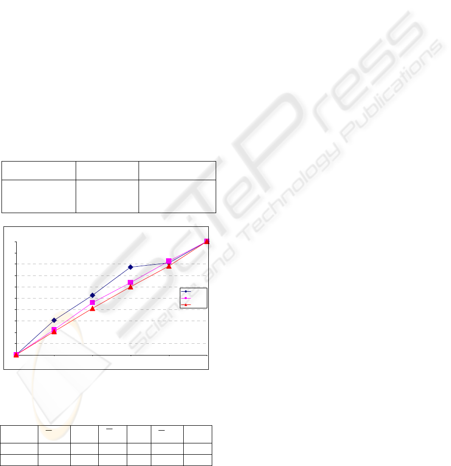
0.01mm, 0.1mm, and 1mm increments for the 3D

tests are presented in Figure 3.

The accuracy in 3D is lower than in the 2D case,

due to calibration and reconstruction errors, and

according to the tests performed it is approximately

1/2 of a pixel.

Table 4 presents the results of the 3D dynamic

tests where the triangle area and side lengths a, b

and c, reconstructed from dynamically-obtained

images were compared to static reconstruction of the

same triangles. 10 triangles were compared, each

formed by a diode in IR-LED array. The average

lengths and the standard deviations are presented.

Table 3: Comparison of standard deviations and R

values

for different moving increments in 3D.

increments [mm]

standard

deviation [mm]

0.01 0.058 0.7806

0.1 0.111 0.9315

1 0.140 0.9974

0,00

0,10

0,20

0,30

0,40

0,50

0,60

0,70

0,80

0,90

1,00

123456

positi on

normal ized

difference

0.01 mm

0.1 mm

1 mm

Figure 3: Pixel difference in the 3D reconstruction.

Table 4: comparison of static and dynamic triangles. All

measurements are in mm.

static 193.04 12.46 89.23 2.77 167.84 12.18

dynamic 193.51 12.43 89.03 2.77 167.52 12.03

We observe a significant standard deviation (up

to 7%) of triangle side lengths which we ascribe to

lens distortions since it is almost the same in the

dynamic and in the static case. The images and the

reconstruction in dynamic conditions vary only a

little in comparison to static ones.

5 CONCLUSIONS

We performed the 2D and 3D accuracy evaluation of

the 3D robot vision system consisting of 2 identical

1 Megapixel cameras. The measurements showed

that the raw static 2D accuracy (without any

subpixel processing approaches and lens distortion

compensation) is confidently as good as 1/5 of a

pixel. However, this is reduced to 1/2 of a pixel

when image positions are reconstructed in 3D due to

reconstruction errors.

In the dynamic case, the comparison to static

conditions showed that no significant error is

introduced with moving markers in both, 2D and 3D

environment. For the speed level of an industrial

robot the accuracy is though not reduced

significantly.

ACKNOWLEDGEMENTS

This work was supported by the European 6th FP

project Adaptive Robots for Flexible Manufacturing

Systems (ARFLEX, 2005-2008) and the Slovenian

Research Agency programme Computing structures

and systems (2004-2008).

REFERENCES

Arflex European FP6 project official home page:

http://www.arflexproject.eu

Faugeras, O., 1992. Three-Dimensional Computer Vision:

A geometric Viewpoint, The MIT Press.

Hutchinson, S., Hager, G., Corke, P.I., 1995. A tutorial on

visual servo control, Yale University Technical Report,

RR-1068.

Papa, G., Torkar, D., 2006. Investigation of LEDs with

good repeatability for robotic active marker systems,

Jožef Stefan Institute technical report, No. 9368.

Robson, D., 2006. Robots with eyes, Imaging and

machine vision-Europe, Vol. 17, pp. 30-31.

Ruf, A., Horaud, R., 1999. Visual servoing of robot

manipulators, Part I: Projective kinematics, INRIA

technical report, No. 3670.

Zhang, Z., 1998. A flexible new Technique for Camera

Calibration, Technical report, MSRTR-98-71.

Zuech, N., 2000. Understanding and applying machine

vision, Marcel Dekker Inc.

ROBOT TCP POSITIONING WITH VISION - Accuracy Estimation of a Robot Visual Control System

215