CONJUGATE GRADIENT TECHNIQUES FOR MULTICHANNEL
ADAPTIVE FILTERING
Lino García Morales and Fernando Juan Berenguer Císcar
Escuela Superior Politécnica,Universidad Europea de Madrid, Tajo S/N, Villaviciosa de Odón, Madrid, Spain
Keywords: Multichannel Adaptive Filtering, System Identification, Optimization Method, Conjugate Gradient,
Partitioned Frequency-Domain Adaptive Filtering.
Abstract: The conjugate gradient is the most popular optimization method for solving large systems of linear
equations. In a system identification problem, for example, where very large impulse response is involved, it
is necessary to apply a particular strategy which diminishes the delay, while improving the convergence
time. In this paper we propose a new scheme which combines frequency-domain adaptive filtering with a
conjugate gradient technique in order to solve a high order multichannel adaptive filter, while being
delayless and guaranteeing a very short convergence time.
1 INTRODUCTION
The multichannel adaptive filtering problem’s
solution depends on the correlation between the
channels, the number of channels and the order and
nature of the impulse responses involved in the
system. The multichannel acoustic echo cancellation
(MAEC) application, for example, can be seen as a
system identification problem with extremely large
impulse responses (depending on the environment
and its reverberation time, the echo paths can be
characterized by FIR filters with thousands of taps).
In these cases a multirate adaptive scheme such a
partitioned block frequency-domain adaptive filter
(PBFDAF) (Páez and García, 1992) is a good
alternative and is widely used in commercial
systems nowadays. However, the convergence speed
may not be fast enough under certain circumstances.
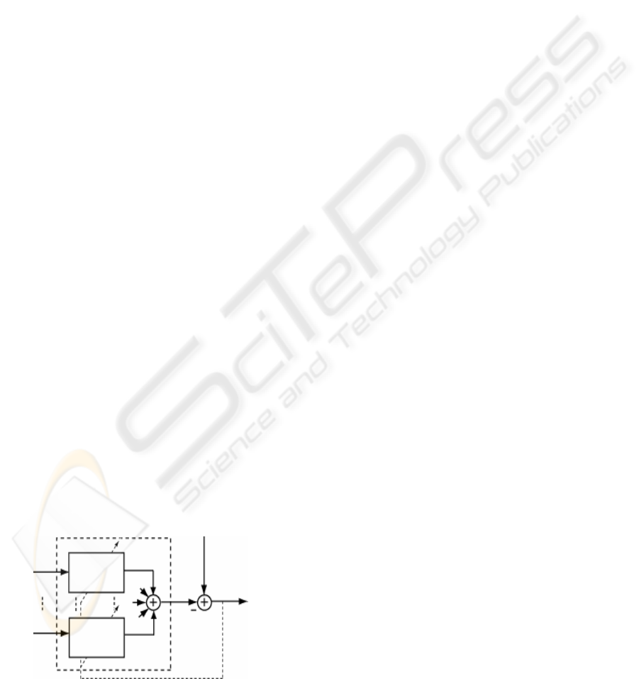
Figure 1: Multichannel Adaptive Filtering.
Figure 1 shows the working framework, where
p
x represents the
p
channel input signal,
d
the
desired signal,
y
the output of adaptive filter and e
the error signal we try to minimize. In typical
scenarios, the filter input signals
p
x , 1, ,
p
P= …
(where
P is a number of channels), are highly
correlated which further reduces the overall
convergence of the adaptive filter coefficients
pm
w ,
1, ,mL
=
… ( L is the filter length),
[] [ ]
11
PL
ppm
pm
y
nxnmw
==
=−
∑∑
.
(1)
The mean square error (MSE) minimization of
the multichannel signal with respect to the filter
coefficients is equivalent to the Wiener-Hopf
equation
=
Rw r .
(2)
R
represents the autocorrelation matrix and
r
the cross-correlation vector between the input and
the desired signals. Both are a priori time-domain
statistical unknown variables, although can be
estimated iteratively from
x and
d
.
x
1
x
P
x
P
w
1
w
y
d
e
17
García Morales L. and Juan Berenguer Císcar F. (2007).
CONJUGATE GRADIENT TECHNIQUES FOR MULTICHANNEL ADAPTIVE FILTERING.
In Proceedings of the Fourth International Conference on Informatics in Control, Automation and Robotics, pages 17-24
DOI: 10.5220/0001644100170024
Copyright
c
SciTePress

{
}
H
E=Rxx and
{
}
*
Ed=rx, with
1
T
TT
P
⎡⎤
=
⎣⎦
xx x… ;
1
T
TT
P
⎡⎤
=
⎣⎦
ww w…
and
1
T
pp pL
ww
⎡⎤
=
⎣⎦
w … . In the notation we
are using
a for scalar, a for vector and A for
matrix;
a
, A denotes vector and matrix
respectively in a frequency-domain:
=
Faa ,
= FAA
.
F
represents the discrete Fourier
transform (DFT) matrix defined as
2jklM
kl
e
π
−
=F ,
with ,0,, 1kl M=−… , 1j =− and
1
−
F as its
inverse. Of course, in the final implementation, the
DFT matrix is substituted by much more efficient
fast Fourier transforms (FFT). Here
()
.
T
denotes
transpose operator and
() ()
()
*
..
HT
= the
Hermitian operator (conjugate transpose).
The conjugate gradient (CG) method is efficient
to obtain the solution to (2), however, a big delay is
introduced (noted that the system order is
LP LP× ). In order to reduce this convergence
speed problem we propose a new algorithm which
employs much more powerful CG optimization
techniques, but keeping the frequency block
partition strategy to allow computationally realistic
low latency situations. The paper is organized as
follows: Section 2 reviews the Multichannel
PBFDAF approach and its implementation. Section
3 develops the Multichannel Conjugate Gradient
Partitioned Frequency Domain Adaptive Filter
algorithm (PBFDAF–CG). Results of the new
approach are presented in Section 4 and 5 followed
by conclusions.
2 PBFDAF
The PBFDAF was developed to deal efficiently with
such situations. The PBFDAF is a more efficient
implementation of Least Mean Square (LMS)
algorithm in the frequency-domain. It reduces the
computational burden and user-delay bounded. In
general, the PBFDAF is widely used due to be good
trade-off between speed, computational complexity
and overall latency. However, when working with
long impulse response, as the acoustic impulse
responses (AIR) used in MAEC, the convergence
properties provided by the algorithm may not be
enough. Besides, the multichannel adaptive filter is
structurally more difficult, in general, than the single
channel case (Benesty and Huang, 2003).
This technique makes a sequential partition of
the impulse response in the time-domain prior to a
frequency-domain implementation of the filtering
operation. This time segmentation allows setting up
individual coefficient updating strategies concerning
different sections of the adaptive canceller, thus
avoiding the need for disabling the adaptation in the
complete filter. The adaptive algorithm is based on
the frequency-domain adaptive filter (FDAF) for
every section of the filter (Shink, 1992).
The main idea of frequency-domain adaptive
filter is to frequency transform the input signal in
order to work with matrix multiplications instead of
dealing with slow convolutions. The frequency-
domain transform employs one or more DFTs and
can be seen as a pre-processing block that generates
decorrelated output signals.
In the more general FDAF case, the output of the
filter in the time domain (1) can be seen as a direct
frequency-domain translation of the block LMS
(BLMS) algorithm. In the PBFDAF case, the filter is
partitioned transversally in an equivalent structure.
Partitioning
p
w in Q segments ( K length) we
obtain
[] [ ]
()
1
11 0
Q
PK
p
pqK m
pqm
yn x n qK mw
−
+
===
=−−
∑∑∑
(3)
Where the total filter length
L , for each channel,
is a multiple of the length of each segment
LQK
=
, KL
≤
. Thus, using the appropriate data
sectioning procedure, the
Q linear convolutions
(per channel) of the filter can be independently
carried out in the frequency-domain with a total
delay of
K samples instead of the QK samples
needed in standard FDAF implementations.
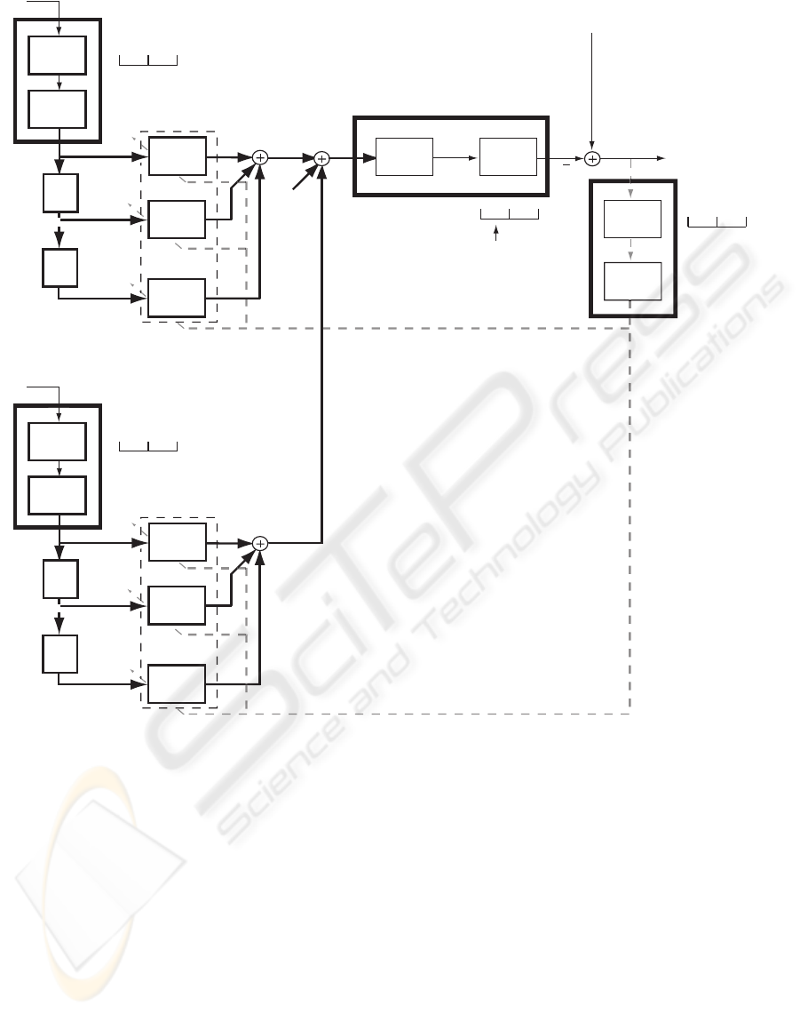
Figure 2 shows the block diagram of the
algorithm using the overlap-save method. In the
frequency domain with matrix notation, equation (3)
can be expressed as
=
⊗YXW.
(4)
Where
=
FX
X
represents a matrix of
dimensions
M
QP
×
× which contains the Fourier
transform of the
Q partitions and P channels of
the input signal matrix
X
.
ICINCO 2007 - International Conference on Informatics in Control, Automation and Robotics
18
FFT
Concatenate
two blocks
IFFT
Save last
block
Insert
zero block
FFT
FFT
reject
Old New
Old New
Concatenate
two blocks
Figure 2: Multichannel PBFDAF (Overlap-Save method).
Being X , 2KP× -dimensional (supposing
50% overlapping between the new block and the
previous one).
It should be taken into account that the algorithm
adapts every K samples. W represents the filter
coefficient matrix adapted in the frequency-domain
(also
M
QP××
-dimensional) while the
⊗
operator multiplies each of the elements one by one;
which in (4) represents a circular convolution.
The output vector
y can be obtained as the
double sum (rows) of the
Y matrix. First we obtain
a
M
P× matrix which contains the output of each
channel in the frequency-domain
p
y ,
1, ,
p
P= … , and secondly, adding all the outputs
we obtain the output of the whole system
y .
Finally, the output in the time-domain is obtained by
using
-1
last components of K=
y
F y .
(5)
Notice that the sums are performed prior to the
time-domain translation. In this way we reduce
(
)
(
)
11PQ
−
− FFTs in the complete filtering
process. As in any adaptive system the error can be
obtained as
=
−ed
y
,
(6)
[]
()
11
T
dmK d m K
⎡
⎤
=+−⎡⎤
⎣⎦
⎣
⎦
d …
.
1
x
1
x
1
x
d
y
e
e
0
e
y
…
P
x
P
x
P
x
K
z
−
K
z
−
K
z
−
K
z
−
11
x
21
x
1Q
x
11
w
21
w
1Q
w
11
y
21
y
1Q
y
1
P
x
2
P
x
QP
x
1
P
w
2
P
w
QP
w
1
P
y
2
P
y
QP
y
1
y
P
y
y
CONJUGATE GRADIENT TECHNIQUES FOR MULTICHANNEL ADAPTIVE FILTERING
19

The error in the frequency-domain (for the
actualization of the filter coefficients) can be
obtained as
1K×
⎡⎤
=
⎢⎥
⎣⎦
0
F
e
e .
(7)
As we can see, a block of
K zeros is added to
ensure a correct linear convolution implementation.
In the same way, for the block gradient estimation, it
is necessary to employ the same error vector in the
frequency-domain for each partition
q and
channel
p
.
This can be achieved by generating an error
matrix
E with dimensions
M
QP×× which
contains replicas of the error vector, defined in (7),
of dimensions
P and Q ( ←Ee in the notation).
The actualization of the weights is performed as
[
]
[
]
[
]
[
]
12mmmm
μ
+= + ⊗WW G.
(8)
The instantaneous gradient is estimated as
*
=− ⊗GXE.
(9)
This is the unconstrained version of the
algorithm which saves two FFTs from the
computational burden at the cost of decreasing the
convergence speed. As we are trying to improve
specifically this parameter we have implemented the
constrained version which basically makes a
gradient projection. The gradient matrix is
transformed into the time-domain and is transformed
back into the frequency-domain using only the first
K elements of G as
K
QP××
⎡⎤
=
⎢⎥
⎣⎦
G
F
0
G
.
(10)
3 PBFDAF–CG
CG algorithm is a technique originally developed to
minimize quadratic functions, as (2), which was later
adapted for the general case (Luenberger, 1984). Its
main advantage is its speed as it converges in a finite
number of steps. In the first iteration it starts
estimating the gradient, as in the steepest descent
(SD) method, and from there it builds successive
directions that create a set of mutually conjugate
vectors with respect to the positively defined
Hessian (in our case, the auto-correlation matrix
R
in the frequency-domain).
In each m-block iteration the conjugate gradient
algorithm will iterate
()
1, , min ,kNK= …
times; where
N represent the memory of the
gradient estimation,
NK
≤
. In a practical system
the algorithm is stopped when it reaches a user-
determined MSE level. To apply this conjugate
gradient approach to the PBFDAF algorithm the
weight actualization equation (8) must be modified
as
[
]
[
]
[
]
1mmm
α
+= +wwv
.
(11)
Where
w
is the coefficient vector of dimension
1
M
QP
×
which results from rearranging matrix
W (in the notation
←
wW). v is a finite R-
conjugated vector set which satisfies
0,
H
ij
ij
=
∀≠vRv . The R-conjugacy property is
useful as the linear independency of the conjugate
vector set allows expanding the
•
w solution as
1
00
0
K
kk kk
k
ααα
−
•
=
=++=
∑
wv v v .
(12)
Starting at any point
0
w of the weighting space,
we can define
00
=
−vg being
00
←gG,
(
)
00
=∇GW,
00
←pP,
()
000
=∇ −PWG.
1kkkk
α
+
=
+ww v
(13)
()
H
kk
k
H
kk k
α
=
−
gv
vgp
(14)
11kk
+
+
←gG,
()
11kk++
=∇GW
11kk
+
+
←pP
,
(
)
111kkk+++
=∇ −PWG
(15)
11kkkk
β
++
=
−+vg v
(16)
(
)
()
11
1
H
kk k
HS
k
H
kk k
β
++
+
−
=
−
gg g
vg g
(17)
ICINCO 2007 - International Conference on Informatics in Control, Automation and Robotics
20

Where
k
p represents the gradient estimated in
kk
−wg. For that, it is necessary to evaluate
()
=⊗ −YX WG, (5), (6), (7) and (9). In order to
be able to generate nonzero direction vectors which
are conjugate to the initial negative gradient vector,
a gradient estimation is necessary (Boray and
Srinath, 1992). This gradient estimation is obtained
by averaging the instantaneous gradient estimates
over
N
past values. The
∇
operator is an
averaging gradient estimation with the current
weights and
N past inputs
X
and d ,
()
1
0
,,
2
kknkn
N
kk kn
n
N
−−
−
−
=
=∇ =
∑
dWX
GW G .
(18)
This alternative approach does not require
knowing neither the Hessian nor the employment of
a linear search. Notice that all the operations (13-17)
are vector operations that keep the computational
complexity low. The equation (17) is known as the
Hestenes-Stiefel method but there are different
approaches for calculating
k
β
: Fletcher-Reeves
(19), Polar-Ribière (20) and Dai-Yuan (21) methods.
11
H
FR
kk
k
H
kk
β
++
=
gg
gg
(19)
()
11
H
kk k
PR
k
H
kk
β
++
−
=
gg g
gg
(20)
()
11
1
H
DY
kk
k
H
kk k
β
++
+
=
−
gg
vg g
(21)
The constant
k
β
is chosen to provide
R
-
conjugacy for the vector
k
v with respect to the
previous direction vectors
10
,,
k −
vv… . Instability
occurs whenever
k
β
exceeds unity.
In this approach, the successive directions are not
guaranteed to be conjugate to each other, even when
one uses the exact value of the gradient at each
iteration. To ensure the algorithm stability the
gradient can be initialized forcing
1
k
β
= in (16)
when
1
k
β
> .
4 COMPUTATIONAL COST
Table 1 shows a comparative analysis for both
algorithms in terms of operations number
(multiplications, sums) clustered by functionality.
Note that constants
A ,
B
and
C
, in the PBFDAF
computational burden estimation, are used as
reference for the number of operations in PBFDAF–
CG. For one iteration (k = 1), the computational cost
of the PBFDAF–CG is 40 times higher than the
PBFDAF.
5 SIMULATION EXAMPLES
MAEC application is a good example of complex
system identification because has to deal with very
long adaptive filters in order to achieve good results.
The scenario employed in our tests simulates two
small chambers imitating a typical teleconference
environment. Following an acoustic opening
approach, both chambers can be acoustically
connected by means of linear arrays of microphones
and loudspeakers. Details of this configuration
follow. Room dimensions are [2000 2440 2700]
mm.
The impulse responses are calculated using the
image method (Allen and Berkley, 1979) with an
expected reverberation time of 70ms (reflection
coefficients [0.8 0.8; 0.5 0.5; 0.6 0.6]). The speech
source, microphones and loudspeakers are situated
as in Figure 3. In the emitting room, the source is
located in [1000 500 1000] and the microphones in
[{800 900 1000 1100 1200} 2000 750]. Notice that
the microphone separation is only 10 cm, which
would be a worse case scenario that provides with
highly correlated signals. In the reception room the
loudspeakers are situated in [{500 750 1000 1250
1500} 100 750] and the microphone in [1000 2000
750].
The directivity patterns of the loudspeakers
([elevation 0º, azimuth -90º, aperture beam 180º])
and the microphones ([0º 90º 180º]) are modified so
that they are face to face. We are considering
5P
=
channels as it is a realistic situation for home
applications; enough for obtaining good spatial
localization and significantly more complex than the
stereo case.
CONJUGATE GRADIENT TECHNIQUES FOR MULTICHANNEL ADAPTIVE FILTERING
21
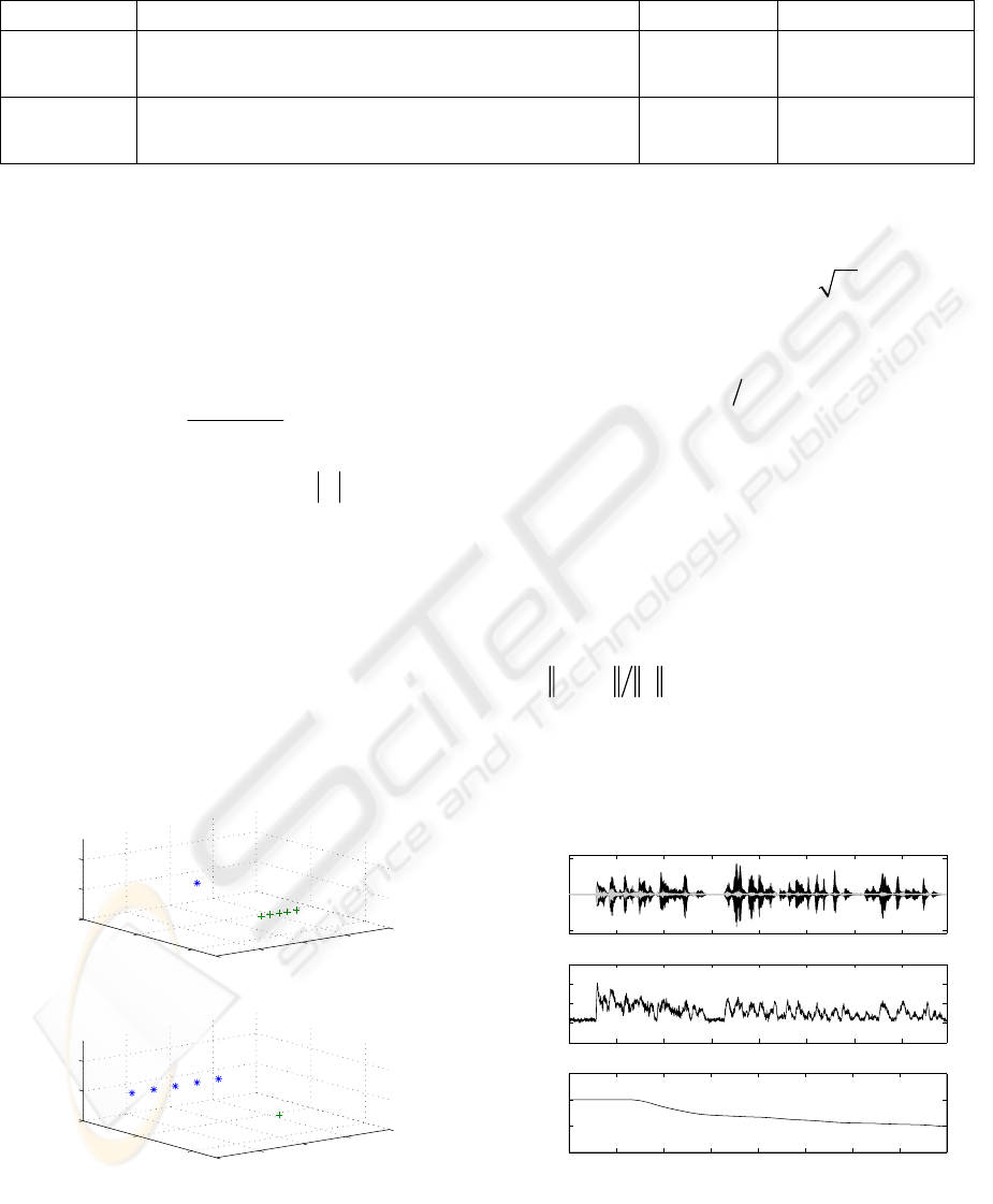
Table 1: Computational Cost Comparative ( OPQM
=
).
Alg.\Op. Gradient Estimation and Convolution Updating Constrained Version
PBFDAF
()
(
)
(
)
2
2log 11
A
POOPQM KO= + + ++++
9
B
O
=
2
2logCO O=
PBFDAF–CG
()
()
(
)
(
)
()
11121 1NA k+++ + +
(
)
13 2Ok+
()
21CN k
+
The source is a male speech recorded in an
anechoic chamber at a sampling rate of 16 kHz and
the background noise in the local room has a power
of -40 dB of SNR.
Figure 4 shows the constrained PBFDAF
algorithm behaviour. For equation (8) we are using a
power normalizing expression as
[]
[]
m
m
μ
μ
δ
=
+
U
,
(22)
[
]
()
[
]
2
11mm
λλ
=− −+UUX.
(23)
Where
[
]
m
μ
is a matrix of dimensions
M
QP××
,
μ
is the step size,
λ
is an averaging
factor, and
δ
is a constant to avoid stability
problems. In our case
0.025
μ
=
, 0.25
λ
= and
0.5
δ
= .
0
500
1000
1500
200
0
0
1000
2000
0
1000
2000
← Microphones
← v01
z−position [mm]
Transmission/Remote room
x−position [mm]
y−position [mm]
0
500
1000
1500
200
0
0
1000
2000
0
1000
2000
← s01
← s02
← s03
← s04
← s05
← Microphone← Microphone
z−position [mm]
Reception/Local room
x−position [mm]
y−position [mm]
← Loudspeakers
Figure 3: Working environment for the tests.
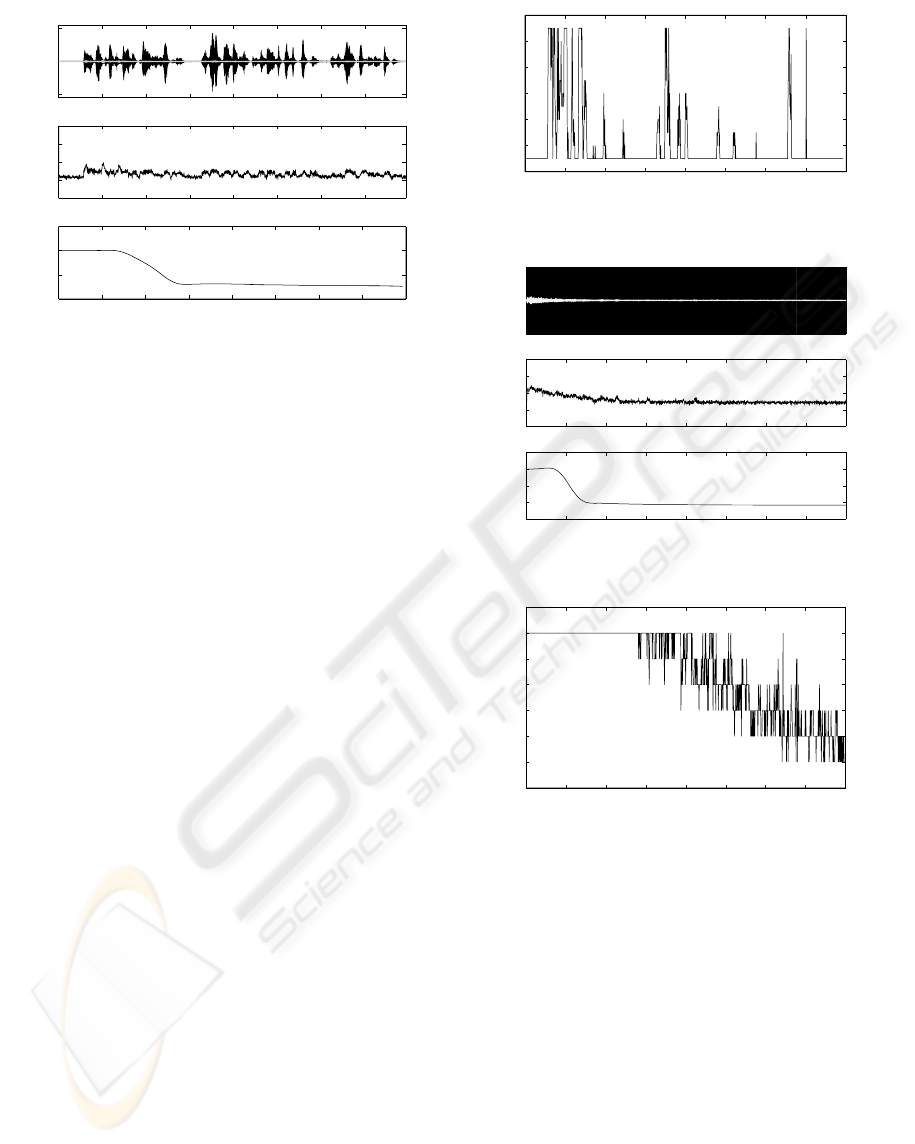
Figure 5 shows the result of using the PBFDAF-
CG algorithm with the Hestenes-Stiefel method
where the difference in convergence can be
observed. A maximum of
NK
⎢⎥
=
⎣⎦
or when
MSE below -45 dB is employed.
For both algorithms we use
8Q = partitions,
1024L
=
taps, 128KLQ
=
= taps for each
partition. The length of the FFTs is
2 256MK
=
= . Working with sample rate of 16
kHz means 8 ms of latency (although a delayless
approach already has been studied) (Bendel and
Burshtein, 2001). Again in both cases the algorithm
uses the overlap-save method (50% overlapping).
The upper part of the figures show the echo
signal
d
(black) and the residual error
e
(grey).
The centre shows the MSE (dB) and the lower
picture the misalignment (also in dB) obtained as
ε
=−hw h, being h the unknown impulse
response and
1
T
TT
P
⎡
⎤
=
⎣
⎦
ww w… the
estimation.
0 1 2 3 4 5 6 7
−1
0
1
d[n](b), e[n](g)
PBFDAF constrained
0 1 2 3 4 5 6 7
−80
−60
−40
−20
0
MSE (dB)
0 1 2 3 4 5 6 7 8
−1
−0.5
0
0.5
misalignment (dB)
time (s)
Figure 4: PBFDAF Constrained.
ICINCO 2007 - International Conference on Informatics in Control, Automation and Robotics
22
0 1 2 3 4 5 6 7
−1
0
1
d[n](b), e[n](g)
PBFDAF−CG constrained
0 1 2 3 4 5 6 7
−80
−60
−40
−20
0
MSE (dB)
0 1 2 3 4 5 6 7 8
−2
−1
0
1
misalignment (dB)
time (s)
Figure 5: PBFDAF–CG Constrained.
The speech input signal to MAEC application is
an inappropriate perturbation signal due to a
nonstationary character. The speech waveform
contains segments of voiced (quasi-periodic) sounds,
such as “e,” unvoiced or fricative (noiselike) sounds,
such as “g,” and silence.
Besides it is possible a double-talk situations
(when the speech of the at least two talkers arrives
simultaneously at the canceller) that made
identification much more problematic than it might
appear at first glance.
A much more conditioned application is an
adaptive multichannel measure of impulse response.
In this case, it is possible to select the best
perturbation signal, with the appropriate SNR, for
system identification and adapt until the error signal
falls below a MSE setting threshold.
The maximum length sequences (MLS) are
pseudorandom binary signals which autocorrelation
function is approximately an impulse.
In an industrial case it is probably the most
convenient method to use because it is simple and
allows system identification without perturbing the
system operation or stopping the plant (Aguado and
Martínez, 2003). In this case it is necessary
superimpose the perturbation signal to the input
system with a power enough to identify the system
while guaranty the optimal functioning.
6 CONCLUSIONS
The PBFDAF algorithm is widely used in
multichannel adaptive filtering applications such as
MAEC commercial systems with good results (in
general for stereo case).
0 1 2 3 4 5 6 7 8
0
2
4
6
8
10
12
Iterations
time (s)
Figure 6: PBFDAF–CG iterations versus time.
0 1 2 3 4 5 6 7 8
−1
0
1
d[n](b), e[n](g)
PBFDAF−CG constrained
0 1 2 3 4 5 6 7 8
−80
−60
−40
−20
0
MSE (dB)
0 1 2 3 4 5 6 7 8
−3
−2
−1
0
1
missaligment (dB)
time (s)
F
igure 7: PBFDAF–CG Constrained (MLS).
0 1 2 3 4 5 6 7 8
5
6
7
8
9
10
11
12
time (s)
iterations
F
igure 8: PBFDAF–CG iterations versus time (MLS).
However, especially when working in
multichannel, high reverberation environments (like
teleconference) its convergence may not be fast
enough. In this article we have presented a novel
algorithm: PFDAF–CG; based on the same structure,
but using much more powerful CG techniques to
speed up the convergence time and improve the
MSE and misalignment performance.
As shown in the results, the proposed algorithm
improves a MSE and misalignment performance,
and converges a lot faster than its counterpart while
keeping the computational convergence relatively
low, because all the operations are performed
between vectors in the frequency-domain. We are
working on better gradient estimation methods in
order to reduce computational cost. Besides, it is
possible to arrive to a compromise between
CONJUGATE GRADIENT TECHNIQUES FOR MULTICHANNEL ADAPTIVE FILTERING
23

complexity and speed modifying the maximum
number of iterations.
Figure 6 shows the PBFDAF–CG iterations
versus time. The total number of iterations for this
experiment is 992 for PBFDAF and 1927 for
PBFDAF–CG (80 times higher computational cost).
Figure 7 shows the result of PBFDAF–CG with
MLS source (identical settings) and Figure 8 the
iterations versus time. Notice that more uniform
MSE convergence and best misalignment. The
computational cost decrease while time the
increases. A better performance is possible
increasing the SNR and diminishing the MSE level
threshold.
REFERENCES
Aguado, A., Martínez, M., 2003. Identificación y Control
Adaptativo, Prentice Hall.
Allen, J.B., Berkley, D.A., 1979. Image method for
efficiently simulating small-room acoustics. In
J.A.S.A., 65:943-950.
Bendel, Y., Burshtein, D., 2001. Delayless Frequency
Domain Acoustic Echo Cancelation. In IEEE
Transactions on Speech and Audio Processing.
9(5):589-587.
Benesty, J., Huang, Y. (Eds.), 2003. Adaptive Signal
Processing: Applications to Real-World Problems,
Springer.
Boray, G., Srinath, M.D., 1992. Conjugate Gradient
Techniques for Adaptive Filtering. In IEEE
Transactions on Circuits and Systems-I: Fundamental
Theory and Application. 39(1):1-10.
Luenberger, D.G., 1984. Introduction to Linear and
Nonlinear Programming, MA: Addison-Wesley,
Reading, Mass.
Shink, J., 1992. Frequency-Domain and Multirate
Adaptive Filtering. In IEEE Signal Processing
Magazine. 9(1):15-37.
Páez Borrallo, J., García Otero, M., 1992. On the
implementation of a partitioned block frequency-
domain adaptive filter (PBFDAF) for long acoustic
echo cancellation. In Signal Processing. 27:301-315.
APPENDIX
The “conjugacy” relation 0,
H
ij
ij=∀≠vRv
means that two vectors,
i
v and
j
v , are orthogonal
with respect to any symmetric positive matrix
R.
This can be looked upon as a generalization of the
orthogonality, for which
R is the unity matrix. The
best way to visualize the working of conjugate
directions is by comparing the space we are working
in with a “stretched” space.
Figure 9: Optimality of CG method.
The SD methods are slow due to the successive
gradient orthogonality that results of minimize the
recursive updating equation (8) respect to
[
]
m
μ
.
The movement toward a minimum has the zigzag
form. The left part in Figure 9 shows the quadratic
function contours in a real space (for
≠r0 in (2)
are elliptical). Any pair of vectors that appear
perpendicular in this space would be orthogonal.
The right part shows the same drawing in a space
that is stretched along the eigenvector axes so that
the elliptical contours from the left part become
circular. Any pair of vectors that appear to be
perpendicular in this space is in fact
R-orthogonal.
The search for a minimum of the quadratic function
starts at
0
w , and takes a step in the direction
0
v
and stops at the point
1
w . This is a minimum point
along that direction, determined in the same way for
SD method. While the SD method would search in
the direction
1
g , the CG method would chose
1
v .
In this stretched space, the direction
0
v appears to
be a tangent to the now circular contours at the point
1
w . Since the next search direction
1
v is
constrained to be
R-orthogonal to the previous, they
will appear perpendicular in this modified space.
Hence,
1
v will take us directly to the minimum
point of the quadratic function (2
nd
order in the
example).
0
w
1
w
0
v
1
v
1
g
w
0
w
w
1
g
1
v
1
w
0
v
ICINCO 2007 - International Conference on Informatics in Control, Automation and Robotics
24
