
TRACKING CONTROL OF WHEELED MOBILE ROBOTS WITH A
SINGLE STEERING INPUT
Control Using Reference Time-Scaling
B
´
alint Kiss and Emese Sz
´
adeczky-Kardoss
Department of Control Engineering and Information Technology
Budapest University of Technology and Economics
Magyar Tud
´
osok krt. 2, Budapest, Hungary
Keywords:
Time-scaling, wheeled mobile robot, flatness, motion planning, tracking control.
Abstract:
This paper presents a time-scaling based control strategy of the kinematic model of wheeled mobile robots
with one input which is the steering angle. The longitudinal velocity of the mobile robot cannot be influenced
by the controller but can be measured. Using an on-line time-scaling, driven by the longitudinal velocity of
the robot and its time derivatives, one can achieve exponential tracking of any sufficiently smooth reference
trajectory with non-vanishing velocity. The price to pay is the modification of the traveling time along the
reference trajectory according to the time-scaling. The measurement of the time derivatives of the velocity is
no longer necessary if the tracking controller is designed to the linearized tracking error dynamics.
1 INTRODUCTION
The kinematic model of a wheeled mobile robot
(WMR) has generally two inputs namely the longitu-
dinal velocity of the rear axis midpoint and the steer-
ing angle of the front wheels. Several strategies are
applied to control such WMRs with these two inputs
including the tracking error transformation based con-
trol reported by (Dixon et al., 2001), the sliding mode
controller based solution proposed by (Benalia et al.,
2003), and the behavior based control strategy studied
by (Gu and Hu, 2002). An important property of the
model is its differential flatness (Fliess et al., 1995;
Fliess et al., 1999) implying its dynamic feedback lin-
earizability (with a singularity at zero velocities).
However, situations may occur where the longitu-
dinal velocity of the WMR is not generated by a feed-
back controller, but by an external source. A practical
example of this scenario is the tracking problem re-
lated to a passenger car without automatic gear. In
such a situation the human driver needs to generate
the velocity of the car with an appropriate manage-
ment of the gas, clutch, and break pedals while the
tracking controller may influence only the angle of
the steered wheels. The kinematic model obtained
in such a situation is no longer differentially, but or-
bitally flat (Respondek, 1998; Guay, 1999), since one
of the inputs is lost.
The control problem is still the tracking of the ref-
erence trajectory but this tracking may become im-
possible if the velocity of the reference WMR mov-
ing along the reference path is always superior to the
real velocity generated by the driver. The opposite is
also possible such that the velocity of the reference
WMR is always inferior to the real velocity gener-
ated by the driver. Nevertheless it is expected that
the path of the controlled WMR joins the path of the
reference WMR for any velocity profile generated by
the driver. To achieve exponential tracking in both
cases, this paper suggests a time-scaling of the refer-
ence path. This time-scaling uses the measurement
of the velocity generated by the driver and eventually
its time derivatives. A practical mean to obtain these
measurements is the use of the ABS signals available
on the CAN bus of the vehicle or the use of alternative
sensors (e.g. accelerometers).
Recall that time-scaling is a commonly used con-
cept to find optimal trajectories, to cope with input
saturation, to reduce tracking errors, and to establish
equivalence classes of dynamical systems.
One may use off-line time-scaling methods to
find the time optimal trajectories for robot manipu-
lators (Hollerbach, 1984) or for autonomous mobile
vehicles (Cuesta and Ollero, 2005). The problem with
these off-line methods is that no sufficient control in-
put margins are always assured for the closed loop
86
Kiss B. and Szádeczky-Kardoss E. (2007).
TRACKING CONTROL OF WHEELED MOBILE ROBOTS WITH A SINGLE STEERING INPUT - Control Using Reference Time-Scaling.
In Proceedings of the Fourth International Conference on Informatics in Control, Automation and Robotics, pages 86-93
DOI: 10.5220/0001644200860093
Copyright
c
SciTePress
control during the tracking. Other algorithms use
therefore on-line trajectory time-scaling for robotic
manipulators to change the actuator boundaries such
that sufficient margin is left for the feedback con-
troller (Dahl and Nielsen, 1990).
Another concept is to use the tracking error in-
stead of the input bounds in order to modify the
time-scaling of the reference path (L
´
evine, 2004;
Sz
´
adeczky-Kardoss and Kiss, 2006). These methods
change the traveling time of the reference path ac-
cording to the actual tracking error by decelerating if
the movement is not accurate enough and by acceler-
ating if the errors are small or vanish.
Time-scaling is also introduced related to the no-
tion of orbital flatness defined in (Fliess et al., 1999)
where a Lie-B
¨
acklund equivalence of dynamical sys-
tems is established such that the transformation in-
volved may change the time according to which the
systems evolve. Another approach that relates time-
scaling to feedback linearization is reported in (Sam-
pei and Furuta, 1986).
The remaining part of the paper is organized as
follows. The next section presents the kinematic mod-
els of the WMRs. Section 3 studies briefly the flatness
properties of the models. Section 4 presents a sim-
ple motion planning method. The time-scaling con-
cept is introduced in Section 5. Two tracking feed-
back laws, both using time-scaling are reported in
Section 6. Simulation results are presented in Sec-
tion 7 and a short conclusion terminates the paper.
2 KINEMATIC WMR MODELS
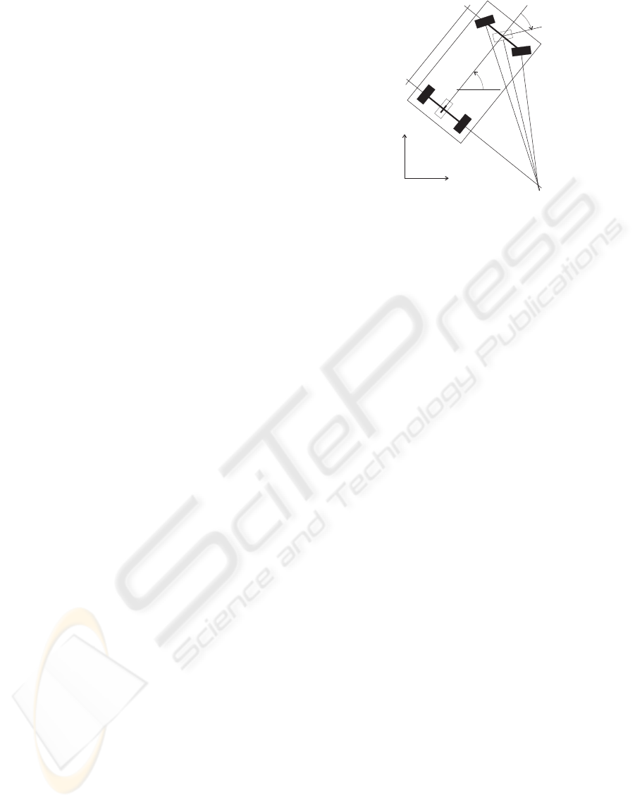
Let us introduce some notations first. Figure 1 depicts
a WMR in the xy horizontal plane. Let us suppose
that the Ackermann steering assumptions hold true,
hence all wheels turn around the same point (denoted
by P) which lies on the line of the rear axle. It follows
that the kinematics of the robot can be fully described
by the kinematics of a bicycle fitted to the longitudinal
symmetry axis of the vehicle (see Figure 1). The co-
ordinates of the rear axle midpoint are given by x and
y. The orientation of the car with respect to the x axis
is denoted by the angle θ, hence the WMR evolves
on the configuration manifold R
2
× S = SE(2). The
angle of the front wheel of the bicycle with respect to
the longitudinal symmetry axis of the robot is denoted
by ϕ. We consider u
2
= ϕ as an input. The longitu-
dinal velocity of the rear axle midpoint is denoted by
u
1
if it is a control input (two input case) and by v
car
if not (one input case).
The distance l between the front and rear axles
equals to one. Then the model equations can be ob-
( )xy,
l
q
j
P
x
y
Figure 1: Notations of the kinematic model.
tained after some elementary considerations which
result (see also for example (Rouchon et al., 1993;
Cuesta and Ollero, 2005))
˙x = u
1
cosθ (1)
˙y = u
1
sinθ (2)
˙
θ = u
1
tanu
2
. (3)
Since time-scaling is involved in the sequel, we pre-
cise that the time in this system is denoted by t and ˙x
denotes the time derivative of the function x(t) such
that
˙
t = 1.
Consider now the case where the longitudinal ve-
locity is not a control input but an external signal v
car
which is generated by the driver or by any other mean
such that the controller has no influence on its evo-
lution. The corresponding model with one input is
defined by the equations
˙x = v
car
cosθ (4)
˙y = v
car
sinθ (5)
˙
θ = v
car
tanu
2
. (6)
Consider now a time different from the time t, de-
noted by τ. Based on (1)-(3), let us define a model
evolving with the time τ and given by the equations
x
′
τ
= u
τ,1
cosθ
τ
(7)
y
′
τ
= u
τ,1
sinθ
τ
(8)
θ
′
τ
= u
τ,1
tanu
τ,2
(9)
where the subscript τ denotes the dependence on the
time τ and x
′
τ
is the derivative of the function x
τ
(τ)
with respect to τ. (No subscript is used for variables
dependent on time t except cases where the distinction
is necessary). It is obvious that τ
′
= 1 as
˙
t = 1.
3 FLATNESS OF THE MODELS
One can easily verify or check in the literature (Rou-
chon et al., 1993; Fliess et al., 1995) that the
TRACKING CONTROL OF WHEELED MOBILE ROBOTS WITH A SINGLE STEERING INPUT - Control Using
Reference Time-Scaling
87

model (1)-(3) (respectively (7)-(9)) is differentially
flat, hence it can be linearized by a dynamic feedback
and a coordinate transformation. The flat output is
given by x and y (respectively x
τ
and y
τ
).
The differential flatness property of the models
can be exploited both for motion planning and track-
ing purposes. Given a reference trajectory x
ref
(t) and
y
ref
(t) for the flat output variables x and y, which are
at least two times differentiable with respect to the
time t, one can determine the time functions of θ
ref
,
u
1,ref
, and u
2,ref
which satisfy (1)-(3) according to a
mapping
{x
ref
,..., ¨x
ref
,y
ref
,..., ¨y
ref
} → {θ
ref
,u
1,ref
,u
2,ref
}.
The same holds true for the model (7)-(9) evolving
with the time τ hence there exists a mapping
{x
τ,ref
,...,x
′′
τ,ref
,y
τ,ref
,...,y
′′
τ,ref
} →
{θ
τ,ref
,u
τ,1,ref
,u
τ,2,ref
}. (10)
The model (4)-(6) is not differentially, but orbitally
flat for v
car
≡ 1 as shown by (Guay, 1999).
4 MOTION PLANNING
The motion planning is done for the system (7)-(9) ex-
ploiting its differential flatness property. The motion
planning realizes the mappings
τ → {x
τ,ref
,x
′
τ,ref
,x
′′
τ,ref
} (11)
τ → {y
τ,ref
,y
′
τ,ref
,y
′′
τ,ref
} (12)
for τ ∈ [0,T] where T is the desired traveling time
along the path such that the mapping (10) allows then
to calculate the time functions of the remaining vari-
ables of the model.
Several motion planning schemes can be used to
realize (11) and (12). One may want to solve an ob-
stacle avoidance problem in parallel with the genera-
tion of the references (Cuesta and Ollero, 2005). For
the sake of simplicity, seventh degree polynomial tra-
jectories are considered in this paper such that
x
τ,ref
=
7
∑
i=0
a
x,i
τ
i
, y
τ,ref
=
7
∑
i=0
a
y,i
τ
i
. (13)
The coefficients are obtained as solutions of a set
of linear algebraic equations determined by the con-
straints that the polynomials and their three succes-
sive derivatives must satisfy at τ = 0 and τ = T. No-
tice that the non-zero constraints are no longer re-
spected in the scaled time t for the derivatives of the
references unless
˙
τ ≡ 1. It follows in particular that
the constraints imposed on the longitudinal velocities
at τ = 0 (respectively at τ = T) will be scaled by
˙
τ(0)
(respectively by
˙
τ(t(T)).
The motion planning can be done off-line prior
to the tracking and the time-scaling does not need
the redesign of the reference. It follows that more
involved methods can be also applied including the
one involving continuous curvature pathes with Fres-
nel integrals (Fraichard and Scheuer, 2004).
5 TIME-SCALING
A time-scaling law, which is defined by the mapping
t 7→ τ(t) or by its inverse τ 7→ t(τ) can be obtained
based on the following consideration. Rewrite (4)-(6)
as
dx = v
car
dt cosθ (14)
dy = v
car
dt sinθ (15)
dθ = v
car
dt tanu
2
. (16)
Similarly, rewrite also (7)-(9) as
dx
τ
= u
τ,1
dτcosθ
τ
(17)
dy
τ
= u
τ,1
dτsinθ
τ
(18)
dθ
τ
= u
τ,1
dτtanu
τ,2
. (19)
Consider now the model equations and the following
relations obtained from (14)-(16) and (17)-(19) for the
inputs of the models
dt
dτ
= t
′
=
u
τ,1
v
car
u
2
= u
τ,2
. (20)
This allows to determine a unique trajectory of the
system (4)-(6) for a trajectory of the system (7)-(9)
if the time function v
car
(t) and the initial conditions
are given, and one supposes non-vanishing velocity
functions v
car
and u
τ,1
. As far as the initial condi-
tions are considered one may, for instance, suppose
that x(0) = x
τ
(0), y(0) = y
τ
(0), θ(0) = θ
τ
(0). The
relations in the other direction are similar and read
dτ
dt
=
˙
τ =
v
car
u
τ,1
u
τ,2
= u
2
. (21)
The following proposition summarizes the properties
of the time-scaling for trajectories with strictly posi-
tive (respectively negative) velocities.
Proposition 1 Suppose that one considers trajecto-
ries of the different models of the kinematic car such
that the velocities v
car
and u
τ,1
are both strictly pos-
itive (respectively strictly negative). Then the time-
scaling t 7→ τ(t) and τ 7→ t(τ) defined by (20)-(21)
satisfying t(0) = τ(0) are such that the functions τ(t)
and t(τ) are strictly increasing functions of their ar-
guments (the scaled time never rewinds).
ICINCO 2007 - International Conference on Informatics in Control, Automation and Robotics
88

This property is a general requirement for mean-
ingful time-scaling and it is satisfied both for forward
and backward motions of the car. The time-scaling
has a singularity if the car is in idle position.
Note that for a fixed velocity time function v
car
(t),
the time-scaling can be influenced by u
τ,1
, one of the
inputs of the flat model evolving with τ. Observe
moreover that for fixed v
car
these relations do not de-
fine a one-to-one correspondence between the sets of
trajectories of the respective systems and the number
of inputs is not preserved, hence they are not Lie-
B
¨
acklund isomorphisms (Fliess et al., 1999).
Suppose that the references are obtained for (7)-
(9) and one disposes of the time functions x
τ,ref
, x
′
τ,ref
,
x
′′
τ,ref
, y
τ,ref
, y
′
τ,ref
, y
′′
τ,ref
. (A simple method is given
in preceding section for the planning of the reference
motion.) The time-scaling is defined by the mappings
{x
τ,ref
,...,x
′′
τ,ref
} → {x
ref
(t),..., ¨x
ref
(t)} (22)
{y
τ,ref
,...,y
′′
τ,ref
} → {y
ref
(t),..., ¨y
ref
(t)} (23)
which can be determined using (21) since
τ(t) =
t
0
v
car
u
ϑ,1
dϑ τ(0) = t(0) = 0 (24)
v
car
=
˙
τu
t,1
(25)
˙v
car
=
¨
τu
t,1
+
˙
τ ˙u
t,1
(26)
allow to express τ(t),
˙
τ, and
¨
τ. Then
x
ref
(t) = x
τ,ref
(τ(t)) (27)
˙x
ref
(t) = x
′
τ,ref
(τ(t))
˙
τ (28)
¨x
ref
(t) = x
′′
τ,ref
(τ(t))
˙
τ
2
+ x
′
τ,ref
(τ(t))
¨
τ (29)
and one obtains similar expressions for the higher or-
der time derivatives and for the mapping (23).
Suppose that a reference trajectory is calculated
according to the time τ and that one is looking for
an open loop control of the real car to follow the ge-
ometry of the reference trajectory. Assume moreover
that the reference trajectory is calculated based on the
initial conditions of the real car. Then the open loop
control signal u
2
(t) can be calculated from the refer-
ence u
τ,2,ref
using the time-scaling defined by (20).
Notice however that the real traveling time for a ref-
erence trajectory according the timet will be obtained
as t(T). If the driver generating v
car
accelerates with
respect to the reference trajectory than T > t(T). If
he/she is more careful than the algorithm providing
the value for T than T < t(T).
6 TRACKING FEEDBACK
DESIGN
Two tracking controllers are presented in this section.
The first one is based on the flatness property of the
model with two inputs and requires the measurement
of the car velocity and its two successive time deriva-
tives. Measurement of the acceleration and its time
derivative may be prohibitive for real applications.
Therefore another tracking feedback is also suggested
which is designed for a system obtained by linearizing
the tracking error dynamics around the reference tra-
jectory achieving only local stability of the reference
trajectory.
6.1 Flatness-Based Tracking using
Time-Scaling
The system (1)-(3) can be linearized by dynamic feed-
back in virtue of its differential flatness property. The
resulting linear system is two chains of integrators
x
(3)
= ω
x
y
(3)
= ω
y
. (30)
Suppose that one specifies the tracking behavior in
terms of the tracking errors e
x
= x − x
ref
and e
y
=
y− y
ref
such that the differential equations
e
(3)
x
+ k
x,2
¨e
x
+ k
x,1
˙e
x
+ k
x,0
e
x
= 0 (31)
e
(3)
y
+ k
y,2
¨e
y
+ k
y,1
˙e
y
+ k
y,0
e
y
= 0 (32)
hold true. The coefficients k
a,i
(a ∈ {x, y}, i = 0,1,2)
are design parameters and have to be chosen such that
the corresponding characteristic polynomials have all
their roots in the left half of the complex plane. These
linear differential equations define another (tracking
feedback) for (30)
ω
x
= x
(3)
ref
− k
x,2
¨e
x
− k
x,1
˙e
x
− k
x,0
e
x
(33)
ω
y
= y
(3)
ref
− k
y,2
¨e
y
− k
y,1
˙e
y
− k
y,0
e
y
. (34)
Consider now the model described by (4)-(6).
This single input model is not differentially flat, hence
cannot be linearized by feedback. It follows that the
flatness property cannot be (directly) used to solve the
tracking problem.
Let us study the possibility to use the time-scaling
defined above to achieve the desired tracking behavior
for the non-differentially flat model (4)-(6) with one
input.
The idea is to use the differentially flat model (7)-
(9) to solve the motion planning problem with the
time τ. Then one would use a tracking feedback con-
troller designed again for the flat model which pro-
duces u
τ,1
and u
τ,2
. The signal u
τ,1
produced by the
controller is used to drive the time-scaling of the ref-
erence trajectory designed for the time τ according
to (21). The control loop is illustrated in Figure 2 for
the model (4)-(6) where the controller provides u
2
= ϕ
to the single input model. The tracking feedback is
TRACKING CONTROL OF WHEELED MOBILE ROBOTS WITH A SINGLE STEERING INPUT - Control Using
Reference Time-Scaling
89
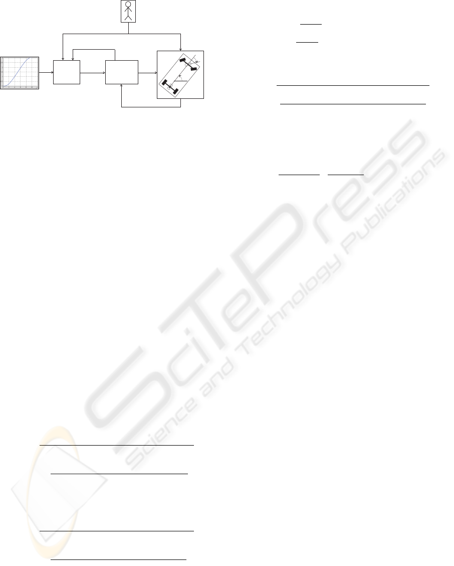
( )xy,
q
j
car
driver
tracking
controller
time
scaling
v
car
ref
in t
ref
in t
u
t,1
j
xy, ,q
motion
planning
Figure 2: Tracking controller with time-scaling.
designed using the flatness property of the model with
two inputs. Define first the dynamics for the feedback
as
˙
ζ
1
= ζ
2
˙
ζ
3
= v
2
(35)
˙
ζ
2
= v
1
ϕ = ζ
3
(36)
u
1
= ζ
1
(37)
where ζ
1
, ζ
2
, and ζ
3
are the (inner) states of the feed-
back. Observe that ζ
2
and v
1
give precisely the deriva-
tives of u
1
which need to realize the time-scaling
in (24)-(26), hence no numerical differentiation is
needed.
The inputs v
1
and v
2
of the feedback dynamics
must be determined such that the tracking errors e
x
(t)
and e
y
(t) satisfy (31) and (32), respectively.
For, one needs to determine first x, ˙x, ¨x, x
(3)
, y, ˙y,
¨y, and y
(3)
as functions of x, y, θ, ζ
1
, ζ
2
, and ζ
3
which
are the states of the closed loop system including the
measured states of the kinematic car model, and the
states of the feedback (35)-(37). After some cumber-
some but elementary differentiations one obtains
˙x = ζ
1
cosθ (38)
¨x = ζ
2
cosθ− ζ
2
1
sinθtanζ
3
(39)
x
(3)
=
v
1
cosθcos
2
ζ
3
−3ζ
1
ζ
2
sinθsinζ
3
cosζ
3
cos
2
ζ
3
−
ζ
3
1
cosθ−ζ
3
1
cosθcos
2
ζ
3
+v
2
ζ
2
1
sinθ
cos
2
ζ
3
(40)
˙y = ζ
1
sinθ (41)
¨y = ζ
2
sinθ+ ζ
2
1
cosθtanζ
3
(42)
y
(3)
=
v
1
sinθcos
2
ζ
3
+3ζ
1
ζ
2
cosθsinζ
3
cosζ
3
cos
2
ζ
3
−
ζ
3
1
sinθ−ζ
3
1
sinθcos
2
ζ
3
−v
2
ζ
2
1
cosθ
cos
2
ζ
3
. (43)
These expressions allow to calculate e
x
, ˙e
x
, ¨e
x
, e
y
, ˙e
y
,
and ¨e
y
using the reference trajectory (scaled with t)
and the states of the closed loop system. Plugging in
these expressions into (31) and (32), and using (30)
one gets
cosθ −
ζ
2
1
sinθ
cos
2
ζ
3
sinθ
ζ
2
1
cosθ
cos
2
ζ
3
v
1
v
2
=
ω
x
−A
ω
y
−B
(44)
with
A
B
=
−3ζ
1
ζ
2
sinθsinζ
3
cosζ
3
−ζ
3
1
cosθ+ζ
3
1
cosθcos
2
ζ
3
cos
2
ζ
3
3ζ
1
ζ
2
cosθsinζ
3
cosζ
3
−ζ
3
1
sinθ+ζ
3
1
sinθcos
2
ζ
3
cos
2
ζ
3
(45)
where the inverse of the coefficient matrix can be cal-
culated symbolically. One obtains
v
1
v
2
=
"
cosθ sinθ
−sinθcos
2
ζ
3
ζ
2
1
cosθcos
2
ζ
3
ζ
2
1
#
ω
x
−A
ω
y
−B
. (46)
The tracking feedback law is defined by (33)-(34),
(35)-(37), and by (46). A singularity occurs if ζ
2
1
=
u
2
1
= 0 which corresponds to zero longitudinal veloc-
ity. Another singular situation corresponds to ζ
3
=
ϕ = u
2
= ±π/2 which may occur if the steered wheels
are perpendicular to the longitudinal axis of the car.
Singularities imply the loss of controllability of the
kinematic car model.
6.2 Linearized Error Dynamics
The above method needed the time derivatives of the
velocity to carry out the time-scaling which may be
difficult to measure or estimate in real application.
The method presented in this section uses a transfor-
mation of the tracking error expressed in the config-
uration variables, and the non-linear model obtained
is linearized around the reference trajectory. The lin-
earized model is controlled by a state feedback similar
to the one reported in (Dixon et al., 2001). The lost
input, which is the longitudinal velocity of the WMR
is again replaced by a virtual input which depends on
the time-scaling of the reference trajectory.
A slightly different kinematic model is used for
this method such that the longitudinal velocity of the
rear axle midpoint and the tangent of the steering an-
gle (u
3
= tanϕ) are the inputs of the mobile robot. If
the one input case is considered, u
3
= tanϕ is the sin-
gle control input.
Suppose, that the desired behavior of the robot
is given by the time functions x
τ,ref
(τ), y
τ,ref
(τ),
θ
τ,ref
(τ) such that these functions identically sat-
isfy (7)-(9) for the corresponding reference input sig-
nals u
τ,1,ref
and u
τ,3,ref
= tanu
τ,2,ref
.
We suggest to scale this reference trajectory ac-
cording to the time t. The scaled reference trajectory
is given by x
ref
(t) = x
τ,ref
(τ), y
ref
(t) = y
τ,ref
(τ), and
ICINCO 2007 - International Conference on Informatics in Control, Automation and Robotics
90
θ
ref
(t) = θ
τ,ref
(τ) and similarly to (7)-(9)
x
′
τ,ref
= u
τ,1,ref
cosθ
τ,ref
(47)
y
′
τ,ref
= u
τ,1,ref
sinθ
τ,ref
(48)
θ
′
τ,ref
= u
τ,1,ref
u
τ,3,ref
. (49)
The tracking errors are defined for the configuration
variables as e
x
= x− x
ref
, e
y
= y− y
ref
, and e
θ
= θ−
θ
ref
. Let us now consider the transformation
e
1
e
2
e
3
=
cosθ sinθ 0
−sinθ cosθ 0
0 0 1
e
x
e
y
e
θ
(50)
of the error vector (e
x
,e
y
,e
θ
) to a frame fixed to the
car such that the longitudinal axis of the car coincides
the transformed x axis. Differentiating this equation
w.r.t. time t and using the general rule ˙a(τ) =
da(τ)
dt
=
∂a
∂τ
∂τ
∂t
= a
′
˙
τ we get the differential equation
˙e
1
˙e
2
˙e
3
=
0 v
car
u
3
0
−v
car
u
3
0 0
0 0 0
e
1
e
2
e
3
+
+
0
sine
3
0
u
τ,1,ref
˙
τ+
w
1
0
0 0
0 w
2
(51)
which describes the evolution of the errors with re-
spect to the reference path. The inputs w
1
and w
2
are
w
1
= v
car
−
˙
τu
τ,1,ref
cose
3
(52)
w
2
= v
car
u
3
−
˙
τu
τ,1,ref
u
τ,3,ref
. (53)
Notice that from these inputs w
1
and w
2
the first
derivative of the time scaling (
˙
τ) and the real input
u
3
= tanϕ can be calculated as
˙
τ =
v
car
− w
1
u
τ,1,ref
cose
3
(54)
u
3
=
w
2
+
˙
τu
τ,1,ref
u
τ,3,ref
v
car
(55)
if the reference value for the longitudinal velocity
u
τ,1,ref
6= 0, the error of the orientation e
3
6= ±π/2,
and the longitudinal velocity of the car v
car
6= 0.
This system can be linearized along the refer-
ence trajectory, i.e. for [
e
1
e
2
e
3
]
T
= 0. The
linearized system is controllable if at least one of
the reference control inputs (u
τ,1,ref
,u
τ,3,ref
) is non-
zero. The setpoint of the linearized system obtained
from (51) can be locally stabilized by a state feedback
of the form
w
1
w
2
= −K
e
1
e
2
e
3
(56)
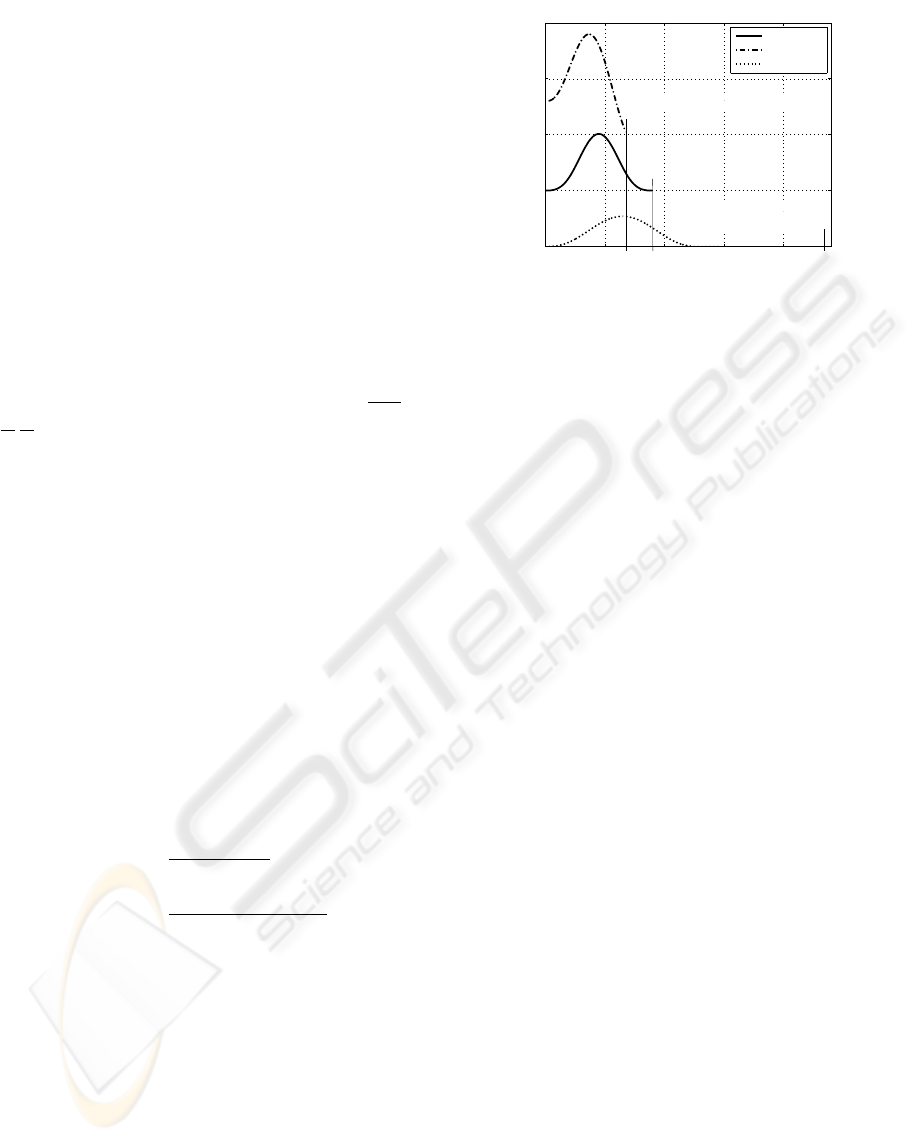
0 5 10 15 20
0.5
1
1.5
2
2.5
time t
velocity [m/s]
Longitudinal velocity profiles
reference
quick driver
slow driver
traveling time of the quick driver
traveling time
of the slow driver
Figure 3: Velocity profiles for the reference, for the quick
driver, and for the slow driver. The traveling times are ob-
tained in closed loop.
such that the gain matrix K puts the eigenvalues of
the closed loop system in the left half of the complex
plane.
The way of calculations is as follows. One sup-
pose that the tracking errors of the configuration vari-
ables (e
x
,e
y
,e
θ
) are measured, hence the the error
(e
1
,e
2
,e
3
) can be determined using (50). Then the
state feedback (56) allows to calculate w
1
and w
2
.
From the actual value of w
1
one can determine
˙
τ using
the current value of v
car
, e
3
, and the value of u
τ,1,ref
according to the time t obtained by scaling the ref-
erence. The input u
3
= tanϕ is calculated according
to (55) using w
2
. The function τ(t) is obtained by the
on-line integration of
˙
τ determined by (54) using the
initial condition τ(0) = 0. The time distribution of the
reference trajectory is finally modified according to τ
and
˙
τ.
Since a linearized model was used for the con-
troller design only local stability is guaranteed. (E.g.
if w
1
≈ 0 is not fulfilled,
˙
τ in (54) can get a negative
value, which is not allowed since time cannot rewind.)
7 SIMULATIONS
Examples are shown to demonstrate the functioning
of both time-scaling based tracking controllers for the
one input case.
7.1 Results of Flatness-Based Solution
We use the feedback described in Subsection 6.1, such
that u
τ,1
generated by the feedback law drives the
time-scaling given in Section 5 together with the mea-
sured v
car
and its two successive time derivatives. The
reference trajectory starts from the point (x
τ,ref
(0) =
0,y
τ,ref
(0) = 0,θ
τ,ref
(0) = 0) and arrives to the point
(x
τ,ref
(T) = 10, y
τ,ref
(T) = 3.5, θ
τ,ref
(T) = 0), all
TRACKING CONTROL OF WHEELED MOBILE ROBOTS WITH A SINGLE STEERING INPUT - Control Using
Reference Time-Scaling
91
−2 0 2 4 6 8 10
0
0.5
1
1.5
2
2.5
3
3.5
x
y
Real and reference trajectories
Real
Reference
Figure 4: Real and reference trajectories in the horizontal
plane – slow driver.
−2 0 2 4 6 8 10 12
0
0.5
1
1.5
2
2.5
3
3.5
4
x
y
Real and reference trajectories
Real
Reference
Figure 5: Real and reference trajectories in the horizontal
plane – quick driver.
distances are given in meters and the orientation is
given in radians. The traveling time of the reference
trajectory is T = 9 seconds.
The real initial configuration of the WMR differs
from the one used for motion planning, since x(0) =
−1.5, y(0) = 2, and θ(0) = π/4.
Two cases are presented such that the geometry
of the reference trajectory and the reference velocity
profile obtained are the same. The driver’s behavior is
different for the two cases. In the first case, referred
to as the slow driver case, the driver imposes con-
siderably slower velocities than those obtained by the
motion planning. In the second case, referred to as the
quick driver case, the driver generates higher veloci-
ties than the reference velocity profile. All velocity
profiles are given in Figure 3.
The geometries of the reference trajectories and
the real trajectories in the horizontal plane are de-
picted in Figure 4 (slow driver) and in Figure 5 (quick
driver). Exponential tracking of the reference trajec-
tory is achieved for each scenario with similar geom-
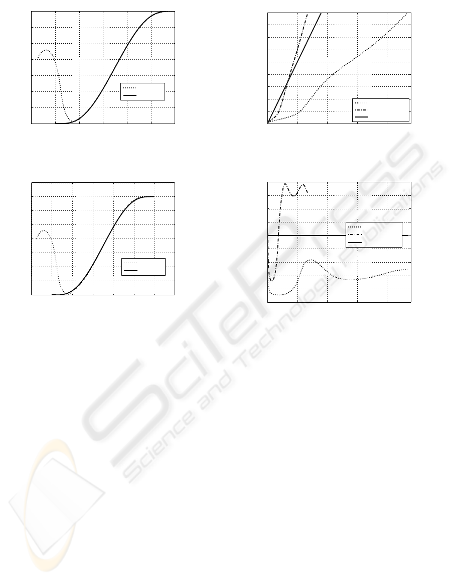
etry of the real path. Figure 6 and Figure 7 show the
effects of on-line time-scaling. If the car is driven by
a slow driver it needed more than 23 seconds accord-
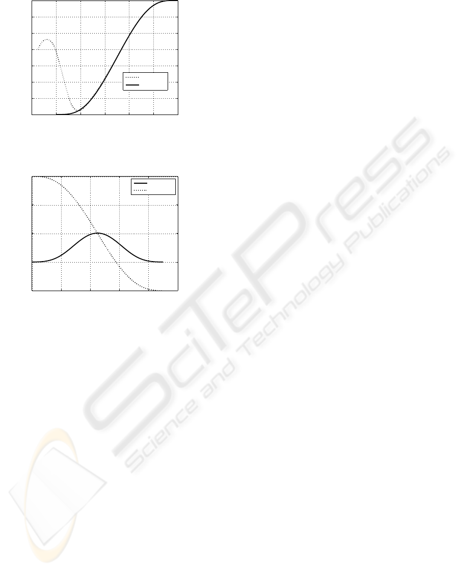
0 5 10 15 20
0
1
2
3
4
5
6
7
8
9
time t
time τ
Time scaling functions τ(t)
slow driver
quick driver
without scaling
Figure 6: The time-scaling functions τ(t) along the path for
the slow and quick drivers.
0 5 10 15 20
0
0.2
0.4
0.6
0.8
1
1.2
1.4
1.6
1.8
time t
Derivative of τ(t)
slow driver
quick driver
without scaling
acceleration of the reference
deceleration of the reference
Figure 7: The derivative of the time-scaling functions
˙
τ.
ing to time t to achieve the traveling time T = 9 sec
which is given for the reference trajectory according
to the time τ. The reference in τ was decelerated all
along the trajectory (
˙
τ < 1). The deceleration is also
accentuated at low values of t which corresponds to
large tracking errors. The time-scaling is completely
different for the quick driver who reaches the end of
the trajectory faster according to the time t than ac-
cording to the time τ which means that the reference
was accelerated except a short section at the begin-
ning where the tracking error elimination slows down
the time-scaling despite the driver’s efforts.
7.2 Results Obtained by State Feedback
Here we use the feedback law described in the sub-
section 6.2 such that the same reference trajectory and
initial configuration were used as in the previous sub-
section.
The reference trajectory and the real path are
shown in Figure 8 for the velocity profiles depicted
in Figure 9. We achieved exponential tracking.
If the difference between the real and reference
initial configurations is larger, the linearized model is
ICINCO 2007 - International Conference on Informatics in Control, Automation and Robotics
92
−2 0 2 4 6 8 10
0
0.5
1
1.5
2
2.5
3
3.5
x
y
Real and reference trajectories
Real
Reference
Figure 8: Real and reference trajectories in the horizontal
plane – simulation 1.
0 2 4 6 8 10
0.5
1
1.5
2
2.5
time t
velocity [m/s]
Longitudinal velocity profiles
Reference
Real
Figure 9: Velocity profiles for the reference and for the car
in simulation 1.
no longer valid and the time-scaling may rewind.
8 CONCLUSION
The paper presented two time-scaling based tracking
control methods for WMRs with one input such that
the longitudinal velocity of the vehicle is generated
externally and cannot be considered as a control in-
put. The time-scaling involves the car velocity and its
derivatives which need to be measured or estimated.
For the tracking controller designed for the linearized
error dynamics the time derivatives of the velocity are
not needed. The exponential decay of the initial error
along the trajectory can be ensured. The results can
be extended for the n-trailer case.
ACKNOWLEDGEMENTS
The research was partially supported by the Hun-
garian Science Research Fund under grant OTKA T
068686 and by the Advanced Vehicles and Vehicle
Control Knowledge Center under grant RET 04/2004.
REFERENCES
Benalia, A., Djemai, M., and Barbot, J.-P. (2003). Control
of the kinematic car using trajectory generation and
the high order sliding mode control. In Proceedings of
the IEEE International Conference on Systems, Man,
and Cybernetics, volume 3, pages 2455–2460.
Cuesta, F. and Ollero, A. (2005). Intelligent Mobile Robot
Navigation, volume 16 of Springer Tracts in Ad-
vanced Robotics. Springer, Heidelberg.
Dahl, O. and Nielsen, L. (1990). Torque-Limited Path Fol-
lowing by On-Line Trajectory Time Scaling. IEEE
Trans. Robot. Automat., 6(5):554–561.
Dixon, W. E., Dawson, D. M., Zergeroglu, E., and Be-
hal, A. (2001). Nonlinear Control of Wheeled Mobile
Robots. In Lecture Notes in Control and Information
Sciences. Springer.
Fliess, M., L
´
evine, J., Martin, P., and Rouchon, P. (1995).
Flatness and Defect of Nonlinear Systems: Intro-
ductory Theory and Examples. Int. J. of Control,
61(6):1327–1361.
Fliess, M., L
´
evine, J., Martin, P., and Rouchon, P. (1999). A
Lie-B
¨
acklund Approach to Equivalence and Flatness
of Nonlinear Systems. IEEE Trans. Automat. Contr.,
44(5):922–937.
Fraichard, T. and Scheuer, A. (2004). From Reeds and
Shepps to Continuous-Curvature paths. IEEE Trans-
action on Robotics and Automation, 20.
Gu, D. and Hu, H. (2002). Neural Predictive Control for
a Car-like Mobile Robot. Robotics and Autonomous
Systems, 39:73–86.
Guay, M. (1999). An Algorithm for Orbital Feedback
Llinearization of Single-Input Control Affine Sys-
tems. Systems and Control Letters, 38:271–281.
Hollerbach, J. M. (1984). Dynamic Scaling of Manipula-
tor Trajectories. Trans. of the ASME, J. of Dynamic
Systems, Measurement, and Control, 106(1):102–106.
L
´
evine, J. (2004). On the Synchronization of a Pair of Inde-
pendent Windshield Wipers. IEEE Trans. Contr. Syst.
Technol., 12(5):787–795.
Respondek, W. (1998). Orbital Feedback Linerization of
Single-Input Nonlinear Control Systems. In Proceed-
ings of the IFAC NOLCOS’98, pages 499–504, En-
schede, The Netherlands.
Rouchon, P., Fliess, M., L
´
evine, J., and Martin, P. (1993).
Flatness and Motion Planning: The Car with n-
Trailers. In ECC’93, Proceedings of the European
Control Conference, pages 1518–1522.
Sampei, M. and Furuta, K. (1986). On Time Scaling
for Nonlinear Systems: Application to Lineariza-
tion. IEEE Transactions on Automatic Control, AC-
31:459–462.
Sz
´
adeczky-Kardoss, E. and Kiss, B. (2006). Tracking Er-
ror Based On-Line Trajectory Time Scaling. In INES
2006, Proc. of 10th Int. Conf. on Intelligent Engineer-
ing Systems, pages 80–85.
TRACKING CONTROL OF WHEELED MOBILE ROBOTS WITH A SINGLE STEERING INPUT - Control Using
Reference Time-Scaling
93
