
CALIBRATION OF QUASI-ISOTROPIC PARALLEL
KINEMATIC MACHINES: ORTHOGLIDE
Anatoly Pashkevich, Roman Gomolitsky
Robotic Laboratory, Department of Control Systems
Belarusian State University of Informatics and Radioelectronics
6 P.Brovka St., Minsk 220027, Belarus
Philippe Wenger, Damien Chablat
Institut de Recherche en Communications et Cybernétique de Nantes
1, rue de la Noe B.P. 6597, 44321 Nantes Cedex 3, France
Keywords: Parallel robots, calibration, parameter identification, error compensation.
Abstract: The paper proposes a novel approach for the geometrical model calibr
ation of quasi-isotropic parallel
kinematic mechanisms of the Orthoglide family. It is based on the observations of the manipulator leg
parallelism during motions between the specific test postures and employs a low-cost measuring system
composed of standard comparator indicators attached to the universal magnetic stands. They are
sequentially used for measuring the deviation of the relevant leg location while the manipulator moves the
TCP along the Cartesian axes. Using the measured differences, the developed algorithm estimates the joint
offsets and the leg lengths that are treated as the most essential parameters. Validity of the proposed
calibration technique is confirmed by the experimental results.
1 INTRODUCTION
Parallel kinematic machines (PKM) are commonly
claimed as appealing solutions in many industrial
applications due to their inherent structural rigidity,
good payload-to-weight ratio, high dynamic
capacities and high accuracy (Tlusty et al., 1999;
Merlet, 2000; Wenger et al., 2001). However, while
the PKM usually exhibit a much better repeatability
compared to serial mechanisms, they may not
necessarily posses a better accuracy, which is
limited by manufacturing/assembling errors in
numerous links and passive joints (Wang and
Masory, 1993). Thus, the PKM accuracy highly
relies on the accurate kinematic model, which must
be carefully tuned for each manipulator separately.
Similar to the serial manipulators, the PKM
cal
ibration techniques are based on the minimization
of a parameter-dependent error function, which
incorporates residuals of the kinematic equations.
For the parallel manipulators, the inverse kinematic
equations are considered computationally more
efficient (contrary to the direct kinematics, which is
usually analytically unsolvable for the PKM)
(Innocenti, 1995; Iurascu & Park, 2003; Jeong et al.,
2004, Huang et al., 2005). But the main difficulty
with this technique is the full-pose measurement
requirement, which is very hard to implement
accurately. Hence, a number of studies have been
directed at using the subset of the pose measurement
data, which however creates another problem, the
identifiability of the model parameters.
Popular approaches in the parallel robot
cal
ibration deal with one-dimensional pose errors
using a double-ball-bar system or other measuring
devices, as well as imposing mechanical constraints
on some elements of the manipulator (Daney, 2003).
However, in spite of hypothetical simplicity, it is
hard to implement in practice since an accurate extra
mechanism is required to impose these constraints.
Additionally, such methods reduce the workspace
size and consequently the identification efficiency.
Another category of the methods, the self- or
au
tonomous calibration, is implemented by
84
Pashkevich A., Gomolitsky R., Wenger P. and Chablat D. (2007).
CALIBRATION OF QUASI-ISOTROPIC PARALLEL KINEMATIC MACHINES: ORTHOGLIDE.
In Proceedings of the Fourth International Conference on Informatics in Control, Automation and Robotics, pages 84-91
DOI: 10.5220/0001646000840091
Copyright
c
SciTePress
minimizing the residuals between the computed and
measured values of the active and/or redundant joint
sensors. Adding extra sensors at the usually
unmeasured joints is very attractive from
computational point of view, since it allows getting
the data in the whole workspace and potentially
reduces impact of the measurement noise. However,
only a partial set of the parameters may be identified
in this way, since the internal sensing is unable to
provide sufficient information for the robot end-
effector absolute location.
More recently, several hybrid calibration
methods were proposed that utilize intrinsic
properties of a particular parallel machine allowing
extracting the full set of the model parameters (or
the most essential of them) from a minimum set of
measurements. It worth mentioning an innovative
approach developed by Renaud et al. (2004, 2005)
who applied the vision-based measurement system
for the PKM calibration from the leg observations.
In this technique, the source data are extracted from
the leg images, without any strict assumptions on the
end-effector poses. The only assumption is related to
the manipulator architecture (the mechanism is
actuated by linear drives located on the base).
However, current accuracy of the camera-based
measurements is not high enough yet to apply this
method in industrial environment.
This paper extends our previous research
(Pashkevich et al., 2006) and focuses on the
calibration of the Orthoglide-type mechanisms,
which is also actuated by linear drives located on the
manipulator base and admits technique of Renaud et
al. (2004, 2005). But, in contrast to the known
works, our approach assumes that the leg location is
observed for specific manipulator postures, when the
tool-center-point moves along the Cartesian axes.
For these postures and for the nominal Orthoglide
geometry, the legs are strictly parallel to the
corresponding Cartesian planes. So, the deviation of
the manipulator parameters influences on the leg
parallelism that gives the source data for the
parameter identification. The main advantage of this
approach is the simplicity and low cost of the
measuring system that can avoid using computer
vision and is composed of standard comparator
indicators attached to the universal magnetic stands.
The remainder of the paper is organized as
follows. Section 2 describes the manipulator
geometry, its inverse and direct kinematics, and also
contains the sensitivity analysis of the leg
parallelism at the examined postures with respect to
the geometrical parameters. Section 3 focuses on the
parameter identification, with particular emphasis on
the calibration accuracy under the measurement
noise. Section 4 contains experimental results that
validate the proposed technique, while Section 5
summarizes the main contributions.
2 ORTHOGLIDE MECHANISM
2.1 Manipulator Architecture
The Orthoglide is a three degrees-of-freedom
parallel manipulator actuated by linear drives with
mutually orthogonal axes. Its kinematic architecture
is presented in Figure 1 and includes three identical
parallel chains, which will be further referred as
“legs”. Each manipulator leg is formally described
as PRP
a
R - chain, where P, R and P
a
denote the
prismatic, revolute, and parallelogram joints
respectively (Figure 2). The output machinery (with
a tool mounting flange) is connected to the legs in
such a manner that the tool moves in the Cartesian
space with fixed orientation (translational motions).
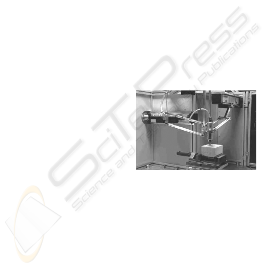
Figure 1: The Orthoglide kinematic architecture.
(© CNRS Photothèque / CARLSON Leif)
The Orthoglide workspace has a regular, quasi-
cubic shape. The input/output equations are simple
and the velocity transmission factors are equal to
one along the x, y and z direction at the isotropic
configuration, like in a conventional serial PPP
machine (Wenger et al., 2000; Chablat and Wenger,
2003). The latter is an essential advantage of the
Orthoglide architecture, which also allows referring
it as the “quasi-isotropic” kinematic machine.
Another specific feature of the Orthoglide
mechanism, which will be further used for the
calibration, is displayed during the end-effector
motions along the Cartesian axes. For example, for
the x-axis motion in the Cartesian space, the sides of
the x-leg parallelogram must also retain strictly
parallel to the x-axis. Hence, the observed deviation
CALIBRATION OF QUASI-ISOTROPIC PARALLEL KINEMATIC MACHINES: ORTHOGLIDE
85
of the mentioned parallelism may be used as the data
source for the calibration algorithms.
P
A
i
ρ
i
B
i
C
i
L
i
d
r
i
i
j
i
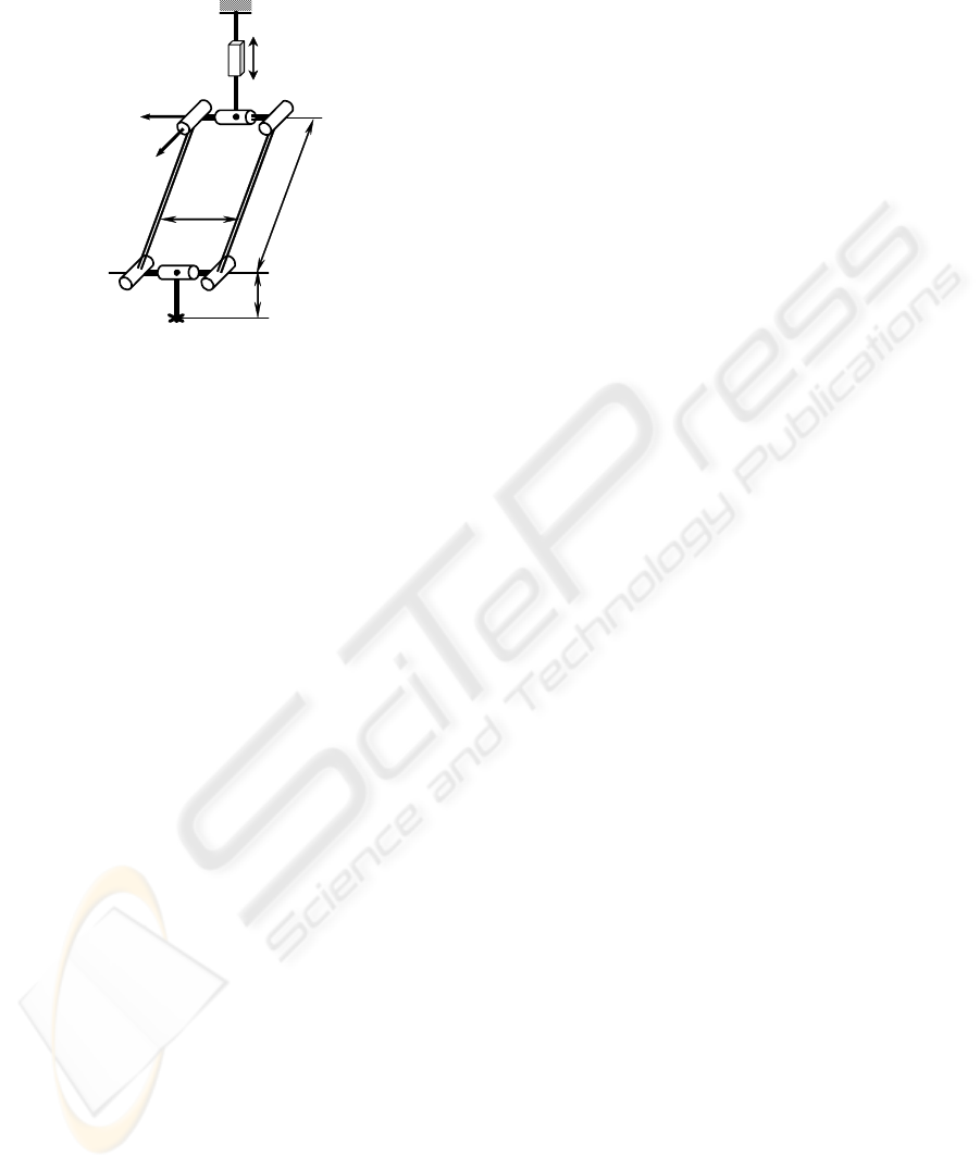
Figure 2: Kinematics of the Orthoglide leg.
For a small-scale Orthoglide prototype used for
the calibration experiments, the workspace size is
approximately equal to 200×200×200 mm
3
with the
velocity transmission factors bounded between 1/2
and 2 (Chablat & Wenger, 2003). The legs nominal
geometry is defined by the following parameters:
L
i
= 310.25 mm, d = 80 mm, r = 31 mm where L
i
, d
are the parallelogram length and width, and r is the
distance between the points Ci and the tool centre
point P (see Figure 2).
2.2 Modelling Assumptions
Following previous studies on the PKM accuracy
(Wang & Massory, 1993; Renaud et al., 2004), the
influence of the joint defects is assumed negligible
compared to the encoder offsets and the link length
deviations. This validates the following modelling
assumptions:
(i) the manipulator parts are supposed to be rigid
bodies connected by perfect joints;
(ii) the manipulator legs (composed of a prismatic
joint, a parallelogram, and two revolute joints)
generate a four degrees-of-freedom motions;
(iii) the articulated parallelograms are assumed to
be perfect but non-identical;
(iv) the linear actuator axes are mutually orthogonal
and intersected in a single point to insure a
translational movement of the end-effector;
(v) the actuator encoders are perfect but located
with some errors (offsets).
Using these assumptions, there will be derived
new calibration equations based on the observation
of the parallel motions of the manipulator legs.
2.3 Basic Equations
Since the kinematic parallelograms are admitted to
be non-identical, the kinematic model developed in
in our previous papers (Pashkevich et al., 2005,
2006) should be extended to describe the
manipulator with different length of the legs.
Under the adopted assumptions, similar to the
equal-leg case, the articulated parallelograms may be
replaced by the kinematically equivalent bar links.
Besides, a simple transformation of the Cartesian
coordinates (shift by the vector (r, r, r)
T
, see Figure
2) allows to eliminate the tool offset. Hence, the
Orthoglide geometry can be described by a
simplified model, which consists of three rigid links
connected by spherical joints to the tool centre point
(TCP) at one side and to the allied prismatic joints at
another side. Corresponding formal definition of
each leg can be presented as PSS, where P and S
denote the actuated prismatic joint and the passive
spherical joint respectively.
Thus, if the origin of a reference frame is located
at the intersection of the prismatic joint axes and the
x, y, z-axes are directed along them, the manipulator
kinematics may be described by the following
equations
⎥
⎥
⎥
⎦
⎤
⎢
⎢
⎢
⎣
⎡
−
++Δ+
=
xx
xxx
xxxxx
L
L
eL
β
βθ
βθρρ
sin
cossin
coscos)(
p
;
(1a)
⎥
⎥
⎥
⎥
⎦
⎤
⎢
⎢
⎢
⎢
⎣
⎡
++Δ+
−
=
yyy
yyyyy
yy
L
eL
L
βθ
βθρρ
β
cossin
coscos)(
sin
p
;
(1b)
⎥
⎥
⎥
⎦
⎤
⎢
⎢
⎢
⎣
⎡
++Δ+
−=
eL
L
L
zzzzz
zz
zzz
βθρρ
β
βθ
coscos)(
sin
cossin
p
,
(1c)
where
p = (p
x
, p
y
, p
z
)
T
is the output vector of the TCP
position,
ρ
= (
ρ
x
,
ρ
y
,
ρ
z
)
T
is the input vector of the
prismatic joints variables, Δ
ρ
= (Δ
ρ
x
, Δ
ρ
y
, Δ
ρ
z
)
T
is
the encoder offset vector, θ
i
, β
i
, i∈{x, y, z} are the
parallelogram orientation angles (internal variables),
and L
i
are the length of the corresponding leg.
After elimination of the internal variables θ
i
, β
i
,
the kinematic model (1) can be reduced to three
equations
(
)
222
2
)(
ikjiii
Lppp =++Δ+−
ρρ
,
(2)
which includes components of the input and output
vectors
p and
ρ
only. Here, the subscripts
ICINCO 2007 - International Conference on Informatics in Control, Automation and Robotics
86
},,{,, zyxkji ∈
,
kji
≠
≠
are used in all
combinations, and the joint variables
ρ
i
are obeyed
the prescribed limits
maxmin
ρ
ρ
ρ
<<
i
defined in
the control software (for the Orthoglide prototype,
ρ
min
= -100 mm and
ρ
max
= +60 mm).
It should be noted that, for the case
0=Δ=Δ=Δ
zyx
ρ
ρ
ρ
and , the
nominal ‘‘mechanical-zero’’ posture of the
manipulator corresponds to the Cartesian
coordinates
p
LLLL
zyx
===
0
= (0, 0, 0)
T
and to the joints variables
ρ
0
= (L, L, L). Moreover, in such posture, the x-, y-
and z-legs are oriented strictly parallel to the
corresponding Cartesian axes. But the joint offsets
and the leg length differences cause the deviation of
the “zero” TCP location and corresponding
deviation of the leg parallelism, which may be
measured and used for the calibration.
Hence, six parameters (Δ
ρ
x
, Δ
ρ
y
, Δ
ρ
z ,
L
x
, L
y
, L
z
)
define the manipulator geometry and are in the focus
of the proposed calibration technique.
2.4 Inverse and Direct Kinematics
The inverse kinematic relations are derived from the
equations (2) in a straightforward way and only
slightly differ from the “nominal” case:
ikjiiii
ppLsp
ρρ
Δ−−−+=
222
,
(3)
where s
x
, s
y
, s
z
∈{ ±1} are the configuration indices
defined for the “nominal” geometry as the signs of
ρ
x
– p
x
, ρ
y
– p
y
, ρ
z
– p
z
, respectively. It is obvious
that expressions (3) give eight different solutions,
however the Orthoglide prototype assembling mode
and the joint limits reduce this set to a single case
corresponding to the s
x
= s
y
= s
z
= 1.
For the direct kinematics, equations (2) can be
subtracted pair-to-pair that gives linear relations
between the unknowns p
x
, p
y
, p
z
, which may be
expressed in the parametric form as
,
)(22
2
ii
i
ii
ii
i
L
t
p
ρρρρ
ρρ
Δ+
−
Δ+
+
Δ+
=
(4)
where t is an auxiliary scalar variable. This reduces
the direct kinematics to the solution of a quadratic
equation with the coefficients
0
2
=++ CBtAt
;)()(
22
∑
≠
Δ+Δ+=
ji
jjii
A
ρρρρ
x
y
z
ρ
x
=
L
+
L
sinα
O
p
ρ
y
=
L
cos
α
ρ
z
=
L
cosα
α
α
(a)
: XMax posture
x
y
z
ρ
x
=
L
O
p
ρ
y
=
L
ρ
z
=
L
(b)
: Zero
posture
x
y
z
ρ
x
=
L
-
L
sinα
O
p
ρ
y
=
L
cos
α
ρ
z
=
L
cosα
α
α
(c)
: XMin
posture
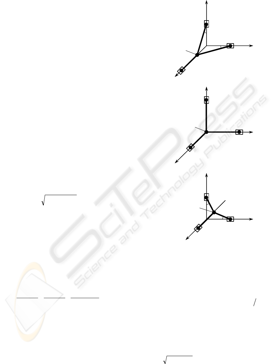
Figure 3: Specific postures of the Orthoglide (for the x-leg
motion along the Cartesian axis X).
;)()()(
2222
kkjj
kji
i
i
ii
LB
ρρρρρρ
Δ+Δ+−Δ+=
∑
∏
≠≠
4/)()(
24/)()(
224
222
kkjj
kji
i
ii
iii
i
ii
L
LC
ρρρρ
ρρρρ
Δ+Δ++
+
⎟
⎟
⎠
⎞
⎜
⎜
⎝
⎛
−Δ+⋅Δ+=
∑
∑∑
∏
≠≠
where
},,{,, zyxkji
∈
. From two possible solutions
that gives the quadratic formula, the Orthoglide
prototype (see Figure 1) admit a single one
AACBBt 2/)4(
2
−+−=
corresponding to the
manipulator assembling mode.
CALIBRATION OF QUASI-ISOTROPIC PARALLEL KINEMATIC MACHINES: ORTHOGLIDE
87
2.5 Differential Relations
To obtain the calibration equations, first let us derive
the differential relations for the TCP deviation for
three types of the Orthoglide postures:
(i) “maximum displacement” postures for the
directions x, y, z (Figure 3a);
(ii) “mechanical zero” or the isotropic posture
(Figure 3b);
(iii) “minimum displacement” postures for the
directions x, y, z (Figure 3c);
These postures are of particular interest for the
calibration since, in the “nominal” case, a
corresponding leg is parallel to the relevant pair of
the Cartesian planes.
The manipulator Jacobian with respect to the
parameters Δ
ρ
=(Δ
ρ
x
, Δ
ρ
y
, Δ
ρ
z
) and L = (
L
x
, L
y
, L
z
)
can be derived by straightforward differentiating of
the kinematic equations (2), which yields
⎥
⎥
⎥
⎦
⎤
⎢
⎢
⎢
⎣
⎡
−
−
−
=
∂
∂
⋅
⎥
⎥
⎥
⎦
⎤
⎢
⎢
⎢
⎣
⎡
−
−
−
zz
yy
xx
zzyx
zyyx
zyxx
ρp
ρp
ρp
ρppp
pρpp
ppρp
00
00
00
ρ
p
⎥
⎥
⎥
⎦
⎤
⎢
⎢
⎢
⎣
⎡
=
∂
∂
⋅
⎥
⎥
⎥
⎦
⎤
⎢
⎢
⎢
⎣
⎡
−
−
−
z
y
x
zzyx
zyyx
zyxx
L
L
L
ρppp
pρpp
ppρp
00
00
00
L
p
.
Thus, after the matrix inversions and
multiplications, the desired Jacobian can be written
as
[]
),();,(),( ρpJρpJρpJ
L
ρ
=
,
(5)
where
1
1
1
1
(.)
−
⎥
⎥
⎥
⎥
⎥
⎥
⎥
⎥
⎦
⎤
⎢
⎢
⎢
⎢
⎢
⎢
⎢
⎢
⎣
⎡
−−
−−
−−
=
zz
y
zz
x
yy
z
yy
x
xx
z
xx
y
ρp
p
ρp
p
ρp
p
ρp
p
ρp
p
ρp
p
ρ
J
1
(.)
−
⎥
⎥
⎥
⎥
⎥
⎥
⎥
⎥
⎦
⎤
⎢
⎢
⎢
⎢
⎢
⎢
⎢
⎢
⎣
⎡
−
−
−
=
z
zz
z
y
z
x
y
z
y
yy
y
x
x
z
x
y
x
xx
L
L
ρp
L
p
L
p
L
p
L
ρp
L
p
L
p
L
p
L
ρp
J
It should be noted that, for the computing
convenience, the above expression includes both the
Cartesian coordinates p
x
, p
y
, p
z
and the joint
coordinates
ρ
x
,
ρ
y
,
ρ
z
, but only one of these sets may
be treated as an independent taking into account the
inverse/direct kinematic relations.
For the “Zero” posture, the differential relations
are derived in the neighbourhood of the point
{p
0
= (0, 0, 0) ; ρ
0
= (L, L, L)}, which after
substitution to (5) gives the Jacobian matrix
⎥
⎥
⎥
⎦
⎤
⎢
⎢
⎢
⎣
⎡
−
−
−
=
100100
010010
001001
0
J
.
(6)
Hence, in this case, the TCP displacement is related
to the joint offsets and the leg legs variations ΔL
i
by
trivial equations
;
iii
Lp
Δ
−
Δ
=
Δ
ρ
.
},,{ zyxi ∈
(7)
For the “XMax” posture, the Jacobian is
computed in the neighbourhood of the point
{
)0,0,(
α
LS
=
p
;
),,(
ααα
LCLCLSL
+
=
ρ
}, where
α is the angle between the y-, z-legs and the X-
axes:
)/sin(
max
La
ρ
α
=
;
)(sin
α
α
=S
,
)cos(
α
α
=C
.
This gives the Jacobian
⎥
⎥
⎥
⎦
⎤
⎢
⎢
⎢
⎣
⎡
−−
−−
−
=
−
−+
1
1
010
001
001001
ααα
ααα
CTT
CTT
x
J
,
(8)
where
)tan(
α
α
=
T
. Hence, the desired equations
for the TCP displacement may be written as
xxx
Lp Δ
−
Δ
=
Δ
ρ
yxyxy
LCLTTp Δ−Δ−Δ+Δ=Δ
−1
ααα
ρρ
zxzxz
LCLTTp Δ−Δ−Δ+Δ=Δ
−1
ααα
ρρ
(9)
It can be proved that similar results are valid for the
“YMax” and “ZMax” postures (differing by the indices
only), and also for the “XMin”, “YMin”, “ZMin” postures.
In the latter case, the angle α should be computed
as
)/sin(
min
La
ρ
α
=
.
3 CALIBRATION METHOD
3.1 Measurement Technique
To evaluate the leg/surface parallelism, we propose
a single-sensor measurement technique. It is based
ICINCO 2007 - International Conference on Informatics in Control, Automation and Robotics
88
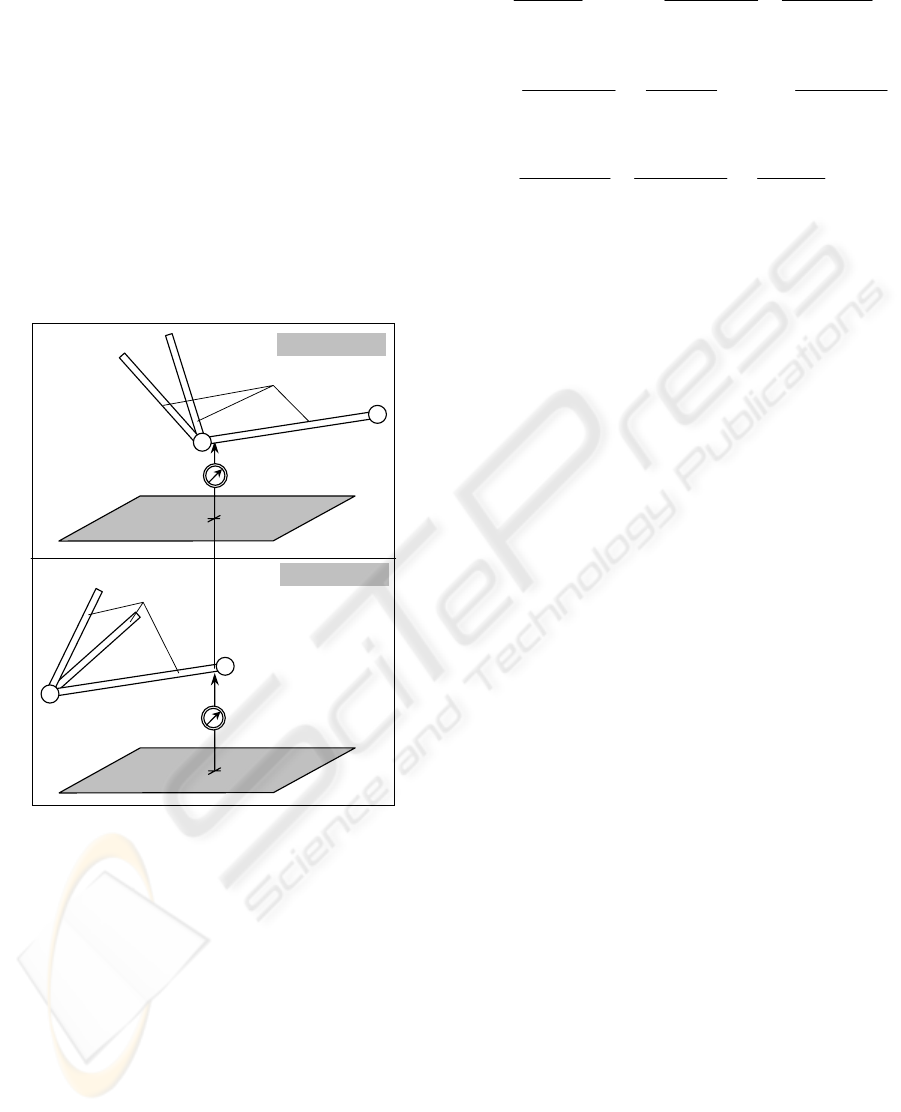
on the fixed location of the measuring device for two
distinct leg postures corresponding to the
minimum/maximum values of the joint coordinates
(Figure 4). Relevant calibration experiment consists
of the following steps:
Step 1. Move the manipulator to the “Zero”
posture; locate two gauges in the middle of the
X-leg (parallel to the axes Y and Z); get their
readings.
Step 2. Move the manipulator to the “XMax” and
“XMin” postures, get the gauge readings, and
compute differences.
Step 3+. Repeat steps 1, 2 for the Y- and Z-legs
and compute corresponding differences.
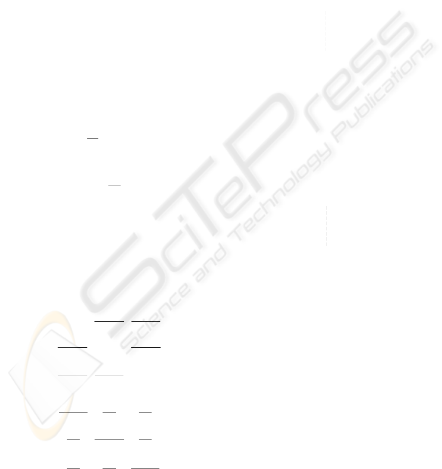
Manipulator legs
d
1
Δ = d
2
-
d
1
Manipulator legs
d
2
Base plane
Base plane
Posture #1
Posture #2
Figure 4: Measuring the leg/surface parallelism.
3.2 Calibration Equations
The system of calibration equations can be derived
in two steps. First, it is required to define the gauge
initial locations that are assumed to be positioned at
the leg middle at the “Zero” posture, i.e. at the points
, where the vectors
r
2/)(
i
rp +
},,{ zyxi ∈
i
define
the prismatic joints centres:
)0;0;(
x
L
x
ρ
Δ+=r
;
;
)0;;0(
y
L
y
ρ
Δ+=r
);0;0(
z
L
z
ρ
Δ+=r
.
Hence, using the equation (7), the gauge initial
locations can be expressed as
⎟
⎟
⎠
⎞
⎜
⎜
⎝
⎛
Δ−Δ
Δ−Δ
Δ+
Δ−
=
2
;
2
;
2
0
zz
yy
x
x
x
L
L
LL
ρ
ρ
ρ
g
⎟
⎟
⎠
⎞
⎜
⎜
⎝
⎛
Δ−Δ
Δ+
Δ−
Δ−Δ
=
2
;
2
;
2
0
zz
y
y
xx
y
L
LL
L
ρ
ρ
ρ
g
⎟
⎟
⎠
⎞
⎜
⎜
⎝
⎛
Δ+
Δ−
Δ−Δ
Δ−Δ
=
z
z
yy
xx
z
LL
L
L
ρ
ρ
ρ
2
;
2
;
2
0
g
Afterwards, in the “XMax”, “YMax”, “ZMax”
postures, the leg location is also defined by two
points, namely, (i) the TCP, and (ii) the centre of the
prismatic joint
r
i
. For example, for the “XMax”
posture, the TCP position is
);;(
max
∗∗Δ−Δ+=
x
L
x
LS
x
ρ
α
p
,
and the joint position is
)0;0;(
max
x
LSL
x
ρ
α
Δ++=r
.
So, the leg is located along the line
maxmax
)1()(
x
x
x
rps ⋅−+⋅=
μμμ
,
where μ is a scalar parameter, μ∈[0, 1]. Since the x-
coordinate of the gauge is independent of the
posture, the parameter μ may be obtained from the
equation
x
x
x
x
]
0
[)]([ gs =
μ
, which solution yields:
L
x
LSS /5.0 Δ⋅
−
+
=
αα
μ
,
Hence, after some transformations, the deviations of
the X-leg measurements (between the “XMax” and
“Zero” postures) may be expressed as
y
LCS
x
LTS
y
S
x
TS
x
y
Δ−
−
+−Δ+−
−Δ+Δ+=
+
Δ
)5.0
1
)5.0(()5.0(
)5.0(
αααα
ρ
α
ρ
αα
z
LCS
x
LTS
z
S
x
TS
x
z
Δ−
−
+−Δ+−
−Δ+Δ+=
+
Δ
)5.0
1
)5.0(()5.0(
)5.0(
αααα
ρ
α
ρ
αα
Similar approach may be applied to the “XMin”
posture, as well as to the corresponding postures for
the Y- and Z-legs. This gives the system of twelve
linear equations in six unknowns:
CALIBRATION OF QUASI-ISOTROPIC PARALLEL KINEMATIC MACHINES: ORTHOGLIDE
89
11 1 1
11 1 1
22 2 2
22 2 2
11 1 1
11 1 1
22 2 2
22 2 2
1111
111 1
2222
2222
00
00
00
00
00
00
00
00
00
00
00
00
x
y
z
x
y
ab c b
ba b c
ab c b
ba b c
ab c b
ba b c
ab c b L
ba b c
L
abcb
bab c
abcb
babc
ρ
ρ
ρ
−−
⎡⎤
⎢⎥
−−
⎢⎥
⎢⎥
−−
⎢⎥
−−
Δ
⎢⎥
⎢⎥
Δ
−−
⎢⎥
⎢⎥
−− Δ
⎢⎥
−− Δ
⎢⎥
⎢⎥
−−
Δ
⎢⎥
Δ
−−
⎢⎥
⎢⎥
−−
⎢⎥
⎢⎥
−−
⎢⎥
−−
⎢⎥
⎣⎦
y
x
y
x
z
y
z
y
z
z
x
z
x
x
y
x
y
y
z
y
z
L
x
z
x
z
+
+
−
−
+
+
−
−
+
+
−
−
⎡⎤
Δ
⎢⎥
Δ
⎢⎥
⎢⎥
Δ
⎢⎥
⎢⎥
Δ
⎡⎤
⎢⎥
⎢⎥
⎢⎥
Δ
⎢⎥
⎢⎥
⎢⎥
⎢⎥
Δ
⎢⎥
=
⎢
⎢⎥
Δ
⎢⎥
⎢⎥
⎢⎥
Δ
⎢⎥
⎢⎥
⎢⎥
⎢⎥
⎣⎦
Δ
⎢⎥
⎢⎥
Δ
⎢⎥
⎢⎥
Δ
⎢⎥
Δ
⎢⎥
⎣⎦
⎥
(10)
where
i
i
Sa
α
=
, ,
ii
i
TSb
αα
+= )5.0(
5.0)5.0(
1
−+=
−
ii
CSc
i
αα
and ,
0)/(asin
max1
>ρ=α L 0)/(asin
min2
<
ρ=α L
.
This system can be solved using the
pseudoinverse of Moore-Penrose, which ensures the
minimum of the residual square sum.
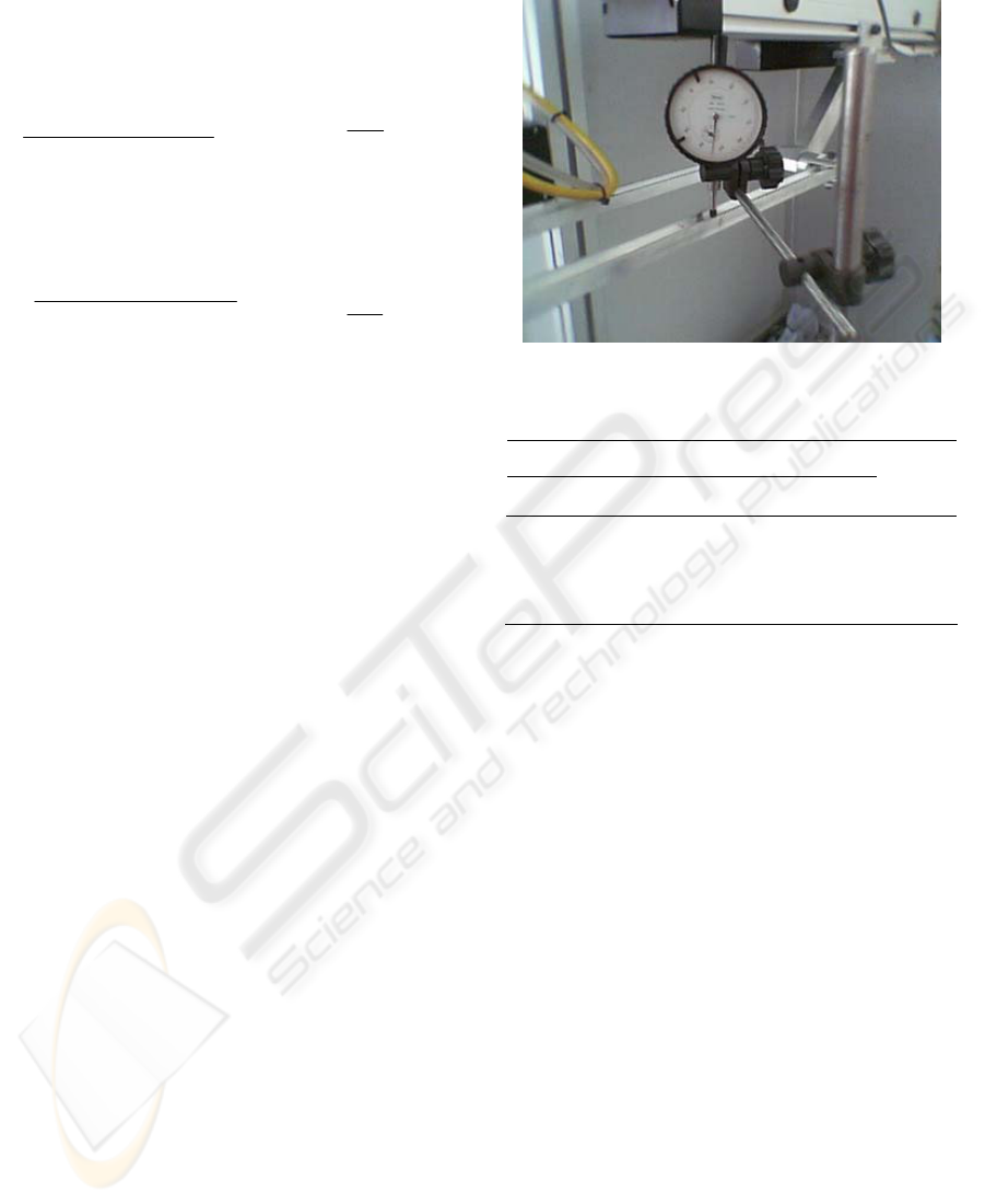
4 EXPERIMENTAL RESULTS
The measuring system is composed of standard
comparator indicators attached to the universal
magnetic stands allowing fixing them on the
manipulator bases. The indicators have resolution of
10 μm and are sequentially used for measuring the
X-, Y-, and Z-leg parallelism while the manipulator
moves between the Max, Min and Zero postures. For
each measurement, the indicators are located on the
mechanism base in such manner that a
corresponding leg is admissible for the gauge
contact for all intermediate postures (Figure 5).
For each leg, the measurements were repeated
three times for the following sequence of motions:
Zero → Max → Min → Zero→ …. Then, the results
were averaged and used for the parameter
identification (the repeatability of the measurements
is about 0.02 mm).
To validate the developed calibration technique
and the adopted modelling assumptions, there were
carried out three experiments targeted to the
following objectives: (#1) validation of modelling
assumptions; (#2) collecting the experimental data
for the parameter identification; and (#3) verification
of the calibration results.
Figure 5: Experimental Setup.
Table 1: Calibration results.
Parameters (mm)
Δ
ρ
x
Δ
ρ
y
Δ
ρ
z
ΔL
x
ΔL
y
ΔL
z
R.m.s.
(mm)
4.66 -5.36 1.46 5.20 -5.96 3.16 0.12
-0.48 0.49 -1.67 – – – 0.14
– – – 0.50 -0.52 1.69 0.14
The first experiment produced rather high
parallelism deviation, which impels to conclude that
the mechanism mechanics requires more careful
tuning. Consequently, the location of the joint axes
was adjusted mechanically to ensure the leg
parallelism for the Zero posture.
The second experiment (after mechanical tuning)
yielded lower deviations, twice better than for the
first experiment. For these data, the developed
calibration algorithm was applied for three sets of
the model parameters: for the full set {Δρ, Δ
L} and
for the reduced sets {Δρ} and {Δ
L}. As follows
from the identification results (Table 1), the
algorithms is able to identify simultaneously both
the joint offsets and Δρ and the link lengths Δ
L.
However, both Δρ and Δ
L (separately) demonstrate
roughly the same influence on the residual
reduction, from 0.32 mm to 0.14 mm, while the full
set {Δρ, Δ
L} gives further residual reduction to the
0.12 mm only. This motivates considering Δρ as the
most essential parameters to be calibrated.
Accordingly, the identified vales of the joint offsets
were input into the control software.
The third experiment demonstrated good
agreement with the expected results. In particular,
the average deviation reduced down to 0.15 mm,
ICINCO 2007 - International Conference on Informatics in Control, Automation and Robotics
90

which corresponds to the measurement accuracy. On
the other hand, further adjusting of the model to the
new experimental data does not give the residual
reduction.
Hence, the calibration results confirm validity of
the proposed identification technique and its ability
to tune the joint offsets and link lengths from
observations of the leg parallelism. Other conclusion
is related to the modelling assumption: for further
accuracy improvement it is prudent to generalize the
manipulator model by including parameters
describing the orientation of the prismatic joint axes,
i.e. relaxing assumption (iv) (see sub-section 2.2).
5 CONCLUSIONS
This paper proposes further developments for a
novel calibration approach for parallel manipulators,
which is based on observations of manipulator leg
parallelism with respect to some predefined planes.
This technique employs a simple and low-cost
measuring system composed of standard comparator
indicators, which are sequentially used for
measuring the deviation of the relevant leg location
while the manipulator moves the TCP along the
Cartesian axes. From the measured differences, the
calibration algorithm estimates the joint offsets and
the link lengths that are treated as the most essential
parameters to be tuned. The validity of the proposed
approach and efficiency of the developed numerical
algorithm were confirmed by the calibration
experiments with the Orthoglide prototype, which
allowed essential reduction of the residuals and
corresponding improvement of the accuracy.
Future work will focus on the expanding the set of
the identified model parameters, their identifiably
analysis, and compensation of the non-geometric
errors.
REFERENCES
Chablat, D., Wenger, Ph., 2003. Architecture Optimization
of a 3-DOF Parallel Mechanism for Machining
Applications, the Orthoglide. IEEE Transactions On
Robotics and Automation, Vol. 19 (3), pp. 403-410.
Daney, D., 2003. Kinematic Calibration of the Gough
platform. Robotica, 21(6), pp. 677-690.
Huang, T., Chetwynd, D.G. Whitehouse, D.J., Wang, J.,
2005. A general and novel approach for parameter
identification of 6-dof parallel kinematic machines.
Mechanism and Machine Theory, Vol. 40 (2), pp. 219-
239.
Innocenti, C., 1995. Algorithms for kinematic calibration
of fully-parallel manipulators. In: Computational
Kinematics, Kluwer Academic Publishers, pp. 241-
250.
Iurascu, C.C. Park, F.C., 2003. Geometric algorithm for
kinematic calibration of robots containing closed
loops. ASME Journal of Mechanical Design, Vol.
125(1), pp. 23-32.
Jeong J., Kang, D., Cho, Y.M., Kim, J., 2004. Kinematic
calibration of redundantly actuated parallel
mechanisms. ASME Journal of Mechanical Design,
Vol. 126 (2), pp. 307-318.
Merlet, J.-P., 2000. Parallel Robots, Kluwer Academic
Publishers, Dordrecht, 2000.
Pashkevich, A., Wenger, P., Chablat, D., 2005. Design
Strategies for the Geometric Synthesis of Orthoglide-
type Mechanisms. Mechanism and Machine Theory,
Vol. 40 (8), pp. 907-930.
Pashkevich A., Chablat D., Wenger P., 2006. Kinematic
Calibration of Orthoglide-Type Mechanisms.
Proceedings of IFAC Symposium on Information
Control Problems in Manufacturing (INCOM’2006),
Saint Etienne, France, 17-19 May, 2006, p. 151 - 156
Renaud, P., Andreff, N., Pierrot, F., Martinet, P., 2004.
Combining end-effector and legs observation for
kinematic calibration of parallel mechanisms. IEEE
International Conference on Robotics and Automation
(ICRA’2004), New-Orleans, USA, pp. 4116-4121.
Renaud, P., Andreff, N., Martinet, P., Gogu, G., 2005.
Kinematic calibration of parallel mechanisms: a novel
approach using legs observation. IEEE Transactions
on Robotics and Automation, 21 (4), pp. 529-538.
Tlusty, J., Ziegert, J.C., Ridgeway, S., 1999. Fundamental
Comparison of the Use of Serial and Parallel
Kinematics for Machine Tools. CIRP Annals, Vol. 48
(1), pp. 351-356.
Wang, J. Masory, O. 1993. On the accuracy of a Stewart
platform - Part I: The effect of manufacturing
tolerances. IEEE International Conference on
Robotics and Automation (ICRA’93), Atlanta,
Georgia, pp. 114–120.
Wenger, P., Gosselin, C., Chablat, D., 2001. Comparative
study of parallel kinematic architectures for machining
applications. In: Workshop on Computational
Kinematics, Seoul, Korea, pp. 249-258.
Wenger, P., Gosselin, C. Maille, B., 1999. A comparative
study of serial and parallel mechanism topologies for
machine tools. In: Proceedings of PKM’99, Milan,
Italy, pp. 23–32.
CALIBRATION OF QUASI-ISOTROPIC PARALLEL KINEMATIC MACHINES: ORTHOGLIDE
91
