AN INVESTIGATION OF EXTENDED KALMAN FILTERING IN
THE ERRORS-IN-VARIABLES FRAMEWORK
A Joint State and Parameter Estimation Approach
Jens G. Linden, Benoit Vinsonneau and Keith J. Burnham
Control Theory and Applications Centre, Coventry University, Priory Street, Coventry, U.K.
Keywords:
Errors-in-variables filtering, Kalman filtering, Parameter estimation.
Abstract:
The paper addresses the problem of errors-in-variables filtering, i.e. the optimal estimation of inputs and
outputs from noisy observations. While the optimal solution is known for linear time-varying systems of
known parameterisation, this paper considers a suboptimal approach where only an approximated set of pa-
rameters is available. The proposed filter is derived by the means of joint state and parameter estimation using
the extended Kalman filter approach which, in turn, leads to a coupled state-parameter estimation procedure.
However, the resulting parameter estimates appear to be biased in the presence of input noise. The novel filter
is compared with a previously proposed suboptimal filter.
1 INTRODUCTION
Kalman filtering (Anderson and Moore, 1979) deals
with the optimal estimation of states and outputs in
the presence of process and output noise. If an errors-
in-variables (EIV) framework is adopted, i.e. the in-
puts are also affected by measurement noise, Kalman
filtering cannot directly be applied (Guidorzi et al.,
2003). The EIV filtering problem, which deals with
the optimal estimation of noise free input and output
signals, has been solved in (Guidorzi et al., 2003) and
(Markovsky and De Moor, 2005). A unified frame-
work for both, Kalman filtering and EIV filtering has
been presented in (Diversi et al., 2005), where the EIV
filtering problem is solved by the means of a standard
Kalman filter (Kf) applied to a reformulated model.
An EIV extended Kalman filter (EIVeKf), which is
able to accommodate for model mismatch, in the case
where the true system generating the data is unknown,
has been presented in (Vinsonneau et al., 2005).
In this paper, the theory of extended Kalman fil-
tering for joint state and parameter estimation (Ljung,
1979) is applied to the reformulated EIV model used
in (Diversi et al., 2005). This leads to an algorithm
which is shown to be similar to the EIVeKf. The dif-
ferences and similarities between both approaches are
discussed. Essentially, the filters calculate an estimate
of the parameters of an assumed model and use this
linear time-varying (LTV) model for filtering. It is re-
vealed that these estimates are biased in the presence
of input noise.
Section 2 reviews the extended Kalman filter for
joint state and parameter estimation, while the exist-
ing EIV filtering techniques are summarised in Sec-
tion 3. The modified algorithm for joint state and pa-
rameter estimation in the case of EIV, which is con-
sidered to be novel, is presented in Section 4, and an
illustrative simulation example is given in Section 5.
In Section 6, both EIV extended Kalman filters are
compared and the results obtained from simulation
are critically appraised . Finally, concluding remarks
are given in Section 7.
2 EKF FOR JOINT STATE AND
PARAMETER ESTIMATION
Assuming the data is generated by a linear time-
invariant (LTI) discrete-time state-space system, its
corresponding model may be given by
x
k+1
= A(θ)x
k
+ B(θ)u
k
+ v
k
(1)
y
k
= C(θ)x
k
+ D(θ)u
k
+ e
k
(2)
47
G. Linden J., Vinsonneau B. and J. Burnham K. (2007).
AN INVESTIGATION OF EXTENDED KALMAN FILTERING IN THE ERRORS-IN-VARIABLES FRAMEWORK - A Joint State and Parameter Estimation
Approach.
In Proceedings of the Fourth International Conference on Informatics in Control, Automation and Robotics, pages 47-53
DOI: 10.5220/0001646600470053
Copyright
c
 SciTePress

where x
k
denotes the state, u
k
the input, y
k
the output,
v
k
process noise, e
k
measurement noise and the model
matrices A(θ), B(θ),C(θ) and D(θ) of appropriate di-
mension are characterised by the parameter vector θ.
The noise sequences
{
v
k
}
and
{
e
k
}
are assumed to be
independent with zero mean and covariance matrices
Σ
v
= E

v
k
v
T
k−τ

δ(τ) (3)
Σ
e
= E

e
k
e
T
k−τ

δ(τ) (4)
Σ
ve
= E

v
k
e
T
k−τ

δ(τ) (5)
where δ(τ) denotes the Kronecker delta function.
Based on an extended Kalman filter (eKf) (Anderson
and Moore, 1979) an adaptive estimator for the model
parameters can be derived by extending the state with
the time dependent parameter vector θ
k
, which leads
to the following nonlinear state equation

x
k+1
θ
k+1

=

A(θ)x
k
+ B(θ)u
k
θ
k

+

v
k
d
k

(6)
The noise term d
k
with covariance matrix
Σ
d
= E

d
k
d
T
k−τ

δ(τ) (7)
allows for variations in the system parameters and is
usually set to zero if time-invariance is assumed.
Defining for convenience
A
k
= A(
ˆ
θ
k
) B
k
= B(
ˆ
θ
k
)
C
k
= C(
ˆ
θ
k
) D
k
= D(
ˆ
θ
k
) (8)
the eKf for joint state and parameter estimation (jeKf)
is given by (Ljung, 1979)
ˆx
k+1
= A
k
ˆx
k
+ B
k
u
k
+ K
k
[y
k
−C
k
ˆx
k
− D
k
u
k
] (9)
ˆ
θ
k+1
=
ˆ
θ
k
+ L
k
[y
k
−C
k
ˆx
k
− D
k
u
k
] (10)
where
K
k
= [A
k
P
1
k
C
T
k
+ F
k
P
T
2
k
C
T
k
+ A
k
P
2
k
H
T
k
+ F
k
P
3
k
H
T
k
+ Σ
ve
]S
−1
k
(11)
S
k
= C
k
P
1
k
C
T
k
+C
k
P
2
k
E
T
k
+ H
k
P
T
2
k
C
T
k
+ H
k
P
3
k
H
T
k
+ Σ
e
(12)
L
k
=

P
T
2
k
C
T
k
+ P
3
k
H
T
k

S
−1
k
(13)
P
1
k+1
= A
k
P
1
k
A
T
k
+ A
k
P
2
k
F
T
k
+ F
k
P
T
2
k
A
T
K
+ F
k
P
3
k
F
T
k
− K
k
S
k
K
T
k
+ Σ
v
(14)
P
2
k+1
= A
k
P
2
k
+ F
k
P
3
k
− K
k
S
k
L
T
k
(15)
P
3
k+1
= P
3
k
− L
k
S
k
L
T
k
+ Σ
d
(16)
with the Jacobians being defined by
F
k
=
∂
∂θ
(A(θ) ˆx
k
+ B(θ)u
k
)


θ=
ˆ
θ
k
(17)
H
k
=
∂
∂θ
(C(θ) ˆx
k
+ D(θ)u
k
)


θ=
ˆ
θ
k
(18)
It is shown in (Ljung, 1979) that the above recursive
parameter estimator can be interpreted as an attempt
to minimise the expected value of squared residuals
associated with a constant model θ, i.e. minimising
the cost function
V(θ) = E
|
¯
ε
k
(θ)
|
2
(19)
where
¯
ε
k
(θ) is the innovation. Hence, this estimator is
closely related to a recursive prediction error method
(Ljung, 1999). A convergence analysis of this param-
eter estimator for linear systems is also carried out in
(Ljung, 1979) and it is shown that it can produce bi-
ased estimates or even diverge. However, the above
procedure can be modified to become a stochastic
descent-algorithm which is globally convergent by in-
cluding an approximation of

∂
∂θ
¯
K(θ)

¯
ε
k
(20)
into the Jacobian F
k
(referred to as the coupling
term (Ljung, 1979)), where
¯
K(θ) is the steady-state
Kalman gain. One way to ensure this is to assume an
innovation model structure
x
k+1
= A(θ)x
k
+ B(θ)u
k
+ K(θ)ε
k
(21)
y
k
= C(θ)x
k
+ D(θ)u
k
+ ε
k
(22)
rather than (1)-(2) and include all elements of
the Kalman gain K into the parameter vector θ.
Parametrising K and Σ
ε
explicitly leads to a modified
algorithm given by
ˆx
k+1
= A
k
ˆx
k
+ B
k
u
k
+ K
k
ε
k
(23)
ˆ
θ
k+1
=
ˆ
θ
k
+ L
k
ε
k
(24)
where
ε
k
= y
k
−C
k
ˆx
k
− D
k
u
k
(25)
L
k
=

P
T
2
k
C
T
k
+ P
3
k
H
T
k

Σ
−1
ε
k
(26)
+ F
k
P
3
k
F
T
k
− K
k
Σ
ε
k
K
T
k
+ Σ
v
(27)
P
2
k+1
= A
k
P
2
k
+ F
k
P
3
k
− K
k
Σ
ε
k
L
T
k
(28)
P
3
k+1
= P
3
k
− L
k
Σ
ε
k
L
T
k
+ Σ
d
(29)
Σ
ε
k
= Σ
ε
k−1
+
1
k

ε
k
ε
T
k
− Σ
ε
k−1

(30)
and
F
k
=
∂
∂θ
(A(θ) ˆx
k
+ B(θ)u
k
+ K(θ)ε
k
)


θ=
ˆ
θ
k
(31)
K
k
= K(
ˆ
θ
k
) (32)
Moreover, a projection facility has to be utilised to
ensure that
ˆ
θ
k
lies in the compact subset
D
s
=
{
θ|A(θ) − K(θ)C(θ) is exponentially stable.
}
(33)
In practice, a step-size reduction might also be neces-
sary to achieve convergence.
ICINCO 2007 - International Conference on Informatics in Control, Automation and Robotics
48

3 KALMAN AND EIV FILTERING
Whereas traditional Kalman filtering (Anderson and
Moore, 1979) addresses the problem of estimating the
optimal states and outputs in the case of process and
output noise, EIV filtering deals with the optimal es-
timation of inputs and outputs, where both quantities
are considered to be observations, which are affected
by additive noise.
The EIV filtering problem for the LTI case has
been solved in (Guidorzi et al., 2003), where the opti-
mal input and output estimates are determined based
on the state-space model
ξ
k+1
=
A ξ
k
+ B

y
T
k
u
T
k

T
(34)
γ
k
=
C ξ
k
+ D

y
T
k
u
T
k

T
(35)
where ξ
k
denotes the state,
A , B , C , D the model ma-
trices and γ
k
the residuals. A different approach has
been presented in (Markovsky and De Moor, 2005),
where the EIV state-space representation is reformu-
lated, such that the new state-space model depends on
the measured quantities u
k
and y
k
with redefined pro-
cess and measurement noise terms. Subsequently, a
modified Kalman filter can be applied to obtain an es-
timate of the system states, which, in turn, allows the
estimation of the true input and output signals. Util-
ising the latter reformulation of the EIV state-space
system, a unified context for both traditional Kalman
filtering and EIV filtering has been proposed (Diversi
et al., 2005) and this is outlined in the following Sub-
section.
3.1 Unified Framework for Kalman and
EIV Filtering
Consider the discrete-time LTI EIV state-space model
given by
x
k+1
= Ax
k
+ Bu
0
k
+ w
k
(36)
y
0
k
= Cx
k
+ Du
0
k
(37)
u
k
= u
0
k
+ ˜u
k
(38)
y
k
= y
0
k
+ ˜y
k
(39)
where x
k
denotes the state, u
0
k
and y
0
k
the unknown
inputs and outputs, u
k
and y
k
the noisy measurements.
The noise terms ˜u
k
, ˜y
k
and w
k
denote input, output
and process noise, respectively, which are assumed to
be of zero mean and with covariance matrices
E

w
k
w
T
k−τ

= Σ
w
δ(τ) (40)
E

˜u
k
˜u
T
k−τ

= Σ
˜u
δ(τ) (41)
E

˜y
k
˜y
T
k−τ

= Σ
˜y
δ(τ) (42)
E

˜u
k
˜y
T
k−τ

= Σ
˜u˜y
δ(τ) (43)
E

w
k
˜u
T
k−τ

= 0 (44)
E

w
k
˜y
T
k−τ

= 0 (45)
The model equations (36)-(39) can be rewritten as
x
k+1
= Ax
k
+ Bu
k
+ v
k
(46)
z
k
= Cx
k
+ e
k
(47)
where z
k
, v
k
and e
k
are the redefined measurements,
process noise and measurement noise, respectively,
which are given by
z
k
= y
k
− Du
k
(48)
and
v
k
= w
k
− B˜u
k
(49)
e
k
= ˜y
k
− D˜u
k
(50)
The covariance matrices are readily obtained via
Σ
v
= Σ
w
+ BΣ
˜u
B
T
(51)
Σ
e
= Σ
˜y
− Σ
T
˜u˜y
D
T
− DΣ
˜u˜y
+ DΣ
˜u
D
T
(52)
Σ
ve
= B

Σ
˜u
D
T
− Σ
˜u˜y

(53)
A standard Kalman filter is then utilised to determine
the optimal state estimate
ˆx
k+1|k
= Ax
k|k−1
+ Bu
k
+ K
k
ε
k
(54)
K
k
=

AP
k|k−1
C
T
+ Σ
ve

Σ
−1
ε
(55)
P
k+1|k
= AP
k|k−1
A
T
+ Σ
v
−

AP
k|k−1
C
T
+ Σ
ve

× Σ
1−
ε

AP
k|k−1
C
T
+ Σ
ve

T
(56)
where
ε
k
= z
k
−Cˆx
k|k−1
= C

x
k
− ˆx
k|k−1

+ e
k
(57)
Σ
ε
= E

ε
k
ε
T
k

= CP
k|k−1
C
T
+ Σ
e
(58)
are the innovations and its corresponding covariance
matrix. The filtered inputs and outputs are then given
by (Diversi et al., 2005)
ˆu
0
k
= u
k
− E [ ˜u
k
|z
k
] = u
k
−

Σ
˜u˜y
− Σ
˜u
D
T

Σ
−1
ε
ε
k
(59)
ˆy
0
k
= y
k
− E [ ˜y
k
|z
k
] = y
k
−

Σ
˜y
− Σ
T
˜u˜y
D
T

Σ
−1
ε
ε
k
(60)
Hence, a traditional Kalman filter can be utilised to
achieve both, the optimal estimation of states and in-
put/output sequences.
AN INVESTIGATION OF EXTENDED KALMAN FILTERING IN THE ERRORS-IN-VARIABLES FRAMEWORK -
A Joint State and Parameter Estimation Approach
49

3.2 Extended EIV Kalman Filtering
A drawback of the linear filter described in Subsec-
tion 3.1, is that it relies on exact information of the
noise characteristics and an exact model of the pro-
cess generating the data. In an attempt to compensate
for the latter requirement, an extended EIV Kalman
filter (EIVeKf), based on the EIV Kalman filter given
in (Guidorzi et al., 2003), has been proposed in (Vin-
sonneau et al., 2005). Instead of an exact process
representation, the EIVeKf requires only an approx-
imate parametrisation of a linear default model, char-
acterised by θ
d
, to achieve acceptable results. Under
certain conditions, use of the EIVeKf can lead to a
superior filter performance with respect to the linear
counterpart in cases where the system parametrisation
is only approximately known. Moreover, the EIVeKf
is also able to accommodate, to a certain degree, the
case of LTV systems.
The idea of the EIVeKf is very similar to the jeKf
approach; the state vector is augmented with the com-
pensating parameters θ
c
such that the new state vector
becomes

ξ
k
θ
c
k

(61)
where ξ
k
is the original state vector in (34) for the cal-
culation of the residual sequence
{
γ
k
}
. The resulting
system equations are thus nonlinear and the EIVKf
filter can be modified using first order Taylor approx-
imations for the predicting step, which results to the
EIVeKf equations.
4 EIV EXTENDED KALMAN
FILTER FOR JOINT
PARAMETER ESTIMATION
Since the EIV filtering problem can be solved by the
means of a standard Kalman filter, as outlined in Sec-
tion 3.1, one could apply well known modifications
of traditional Kalman filtering techniques to estimate
u
0
k
and y
0
k
. The approach proposed here is to ap-
ply the idea of joint state and parameter estimation,
as summarised in Section 2, to EIV systems. This is
expected lead to a similar filter as the one presented in
(Vinsonneau et al., 2005) with the difference that the
estimate
ˆ
θ
k
is not only used for the prediction step, but
in the overall filter equations. In addition, the changes
in the parameters can be tracked by the means of Σ
d
defined in (7).
4.1 Algorithm
Assuming the data is generated by a Eiv system of
structure (36)-(39) and the assumed model structure
is given by
x
k+1
= Ax
k
+ Bu
k
+ v
k
(62)
y
k
= Cx
k
+ Du
k
+ e
k
(63)
with v
k
and e
k
as defined in (49)-(53). Then the EIV
extended Kalman filter for joint parameter estimation
(EIVjeKf) is readily given by (23)-(30) together with
the estimated inputs and outputs as defined in (59) and
(60), whereas A, B, C, D are replaced by A
k
, B
k
, C
k
,
D
k
, respectively.
However, it it found in simulations, that this form
of the EIVjeKf can suffer from outliers in terms of
overall EIV filter performance as illustrated in Section
5. Therefore, a slight different formulation will be
preferred in the subsequent: while the Kalman gain is
still to be estimated, in order to assure the existence of
the terms
h
∂
∂θ
K(θ)
i


θ=
ˆ
θ
k
¯
ε
k
within F
k
, these estimates
are not further utilised in the algorithm but rather K
k
as given by (11)-(16). For clarification, the algorithm
is summarised as follows.
Algorithm 4.1 Assuming an EIV system of the form
(36)-(39) and the model structure of (62)-(63) with
noise characteristics (49)-(53), the EIVjeKf is given
by
1. Augment the state vector x
k
with the model param-
eters θ
k
and Kalman gain K
k
2. Determine the time-varying model matrices A
k
,
B
k
, C
k
and D
k
as given in (8)
3. Compute the innovation given by (25) and its co-
variance matrix as defined in (30)
4. Determine the Jacobians F
k
and H
k
as given in
(31) and (18), respectively
5. Determine the reformulated covariance matrices
(51)-(53) with B and D replaced by B
k
and D
k
6. Compute ˆx
k+1
and
ˆ
θ
k+1
using (9)-(16)
7. Determine ˆu
0
k
and ˆu
0
k
given by (59) and (60),
where D is replaced with D
k
8. Increment k and continue with step 2
Remark 4.1 As outlined in Section 2, the parame-
ter estimator resulting from the EIVjeKf can be inter-
preted as an recursive prediction error method with
the correction inspired by the eKf algorithm. How-
ever, it is known, that the application of standard pre-
diction error methods to EIV systems does not yield
consistent estimates as demonstrated in (S
¨
oderstr
¨
om,
1981). Therefore, the estimated
ˆ
θ
m
is expected to be
biased with respect to the true parametrisation.
ICINCO 2007 - International Conference on Informatics in Control, Automation and Robotics
50

5 SIMULATION
Consider the single-input single-output LTV state-
space system given by (36)-(39) with
A =

0 0.1
−0.2 0.3

B =

0
1

C =

0.9 b
k
− 1.35

D = −4.5 (64)
and
Σ
˜u
= 0.2 Σ
˜y
= 5 Σ
˜u˜y
= 0.8 Σ
w
= 0 (65)
where the time-varying parameter b
k
with mean value
E[b
k
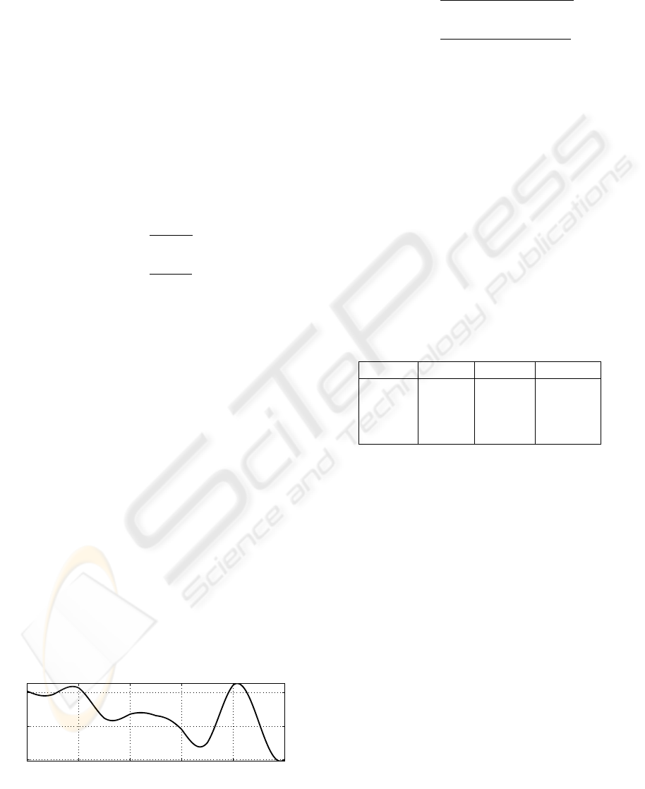
] = 4.7 slowly varies as illustrated in Figure 1.
The input u
0
k
is a zero mean white noise process with
unity variance, the signal-to-noise ratios (SNR) are
given by
SNR
u
= 10log

var(u
0
)
var( ˜u)

= 16.0 (66)
SNR
y
= 10log

var(y
0
)
var(˜y)

= 19.7 (67)
whereas u
0
, ˜u, y
0
, ˜y without index denote the se-
quences to the corresponding signals, i.e. ˜u =
{
˜u
k
}
N
k=1
and so forth. The number of samples is set to N =
5000. While the covariance matrices (65) are as-
sumed to be known, the system parametrisation is ap-
proximated by the default parameter
θ
d
=

−0.5 0.3 −3.1 4.1

T
(68)
while θ
k
is given by
θ
k
=

−0.3 0.2 −4.5 b
k

T
(69)
In order to model the variation in the system pa-
rameters, the covariance matrix (7) corresponding to
θ
k
is chosen to be
Σ
d
=

0
3×3
0
3×1
0
1×3
1· 10
−3

(70)
where 0
m×n
denotes the m × n zero matrix. The per-
formance index of interest is the EIV filter perfor-
mance, i.e ‘how much’ noise can be removed from
1000 2000 3000 4000 5000
2
4
6
samples
amplitude
b
k
Figure 1: Time-varying parameter b
k
.
the noisy observations u
k
and y
k
. This can be quanti-
fied by
P
u
= 100
||
u
0
− u
||
2
−
||
u
0
− ˆu
0
||
2
||
u
0
− u
||
2
(71)
P
y
= 100
||
y
0
− y
||
2
−
||
y
0
− ˆy
0
||
2
||
y
0
− y
||
2
(72)
giving a relative measure for the removed noise in per-
centage, i.e. a value of 100 indicates a perfect filtering
(estimate and true signal are identical), while a value
of 0 corresponds to no filtering performance (estimate
and noisy signal are identical). All simulations are
verified by the means of 100 Monte-Carlo runs.
5.1 Results
The three filters are applied to the above simulation,
that is, the Kf presented in Section 3.1, the EIVeKf
of (Vinsonneau et al., 2005) and the new approach,
the EIVjeKf discussed in the previous Section. The
mean and variances of P
u
and P
y
for the different
Monte-Carlo runs are summarised in Table 1. It is
Table 1: Filter performance for the different filters.
Kf EIVeKf EIVjeKf
E[P
u
] 25.2 33.7 42.9
E[P
y
] 26.1 38.5 50.0
var(P
u
) 0.9 1.4 2.1
var(P
y
) 0.8 0.8 2.5
observed that the Kf exhibits the worst EIV filter per-
formance by removing only around 25% and 26% of
input and output noise, respectively, while the best
performance is achieved applying the EIVjeKf, which
removes on average approximately 43% and 50% of
the noise contamination. In contrast, the variances of
the performance indices with respect to the Monte-
Carlo simulation are smaller in the case of the Kf. The
results of the EIVeKf lie in between of the other two
filters for both, mean and variance of the filter perfor-
mance.
6 DISCUSSION
Since only a default time-invariant model (and not
the true system parametrisation) is available to the
Kf, a negative impact on the filter performance is not
surprising. If the true LTV system parametrisation,
and hence, the true time-varying covariance matrices
(51)-(53) are known, the Kf would be optimal and
may well outperform the eKf approaches considered
AN INVESTIGATION OF EXTENDED KALMAN FILTERING IN THE ERRORS-IN-VARIABLES FRAMEWORK -
A Joint State and Parameter Estimation Approach
51

here. In fact, the only reason that the nonlinear ap-
proaches yield superior performance is that they at-
tempt to compensate for the parameter-mismatch by
estimating the the model parameters, which are then
used for filtering (at least in-part).
The different performance results of the EIVeKf
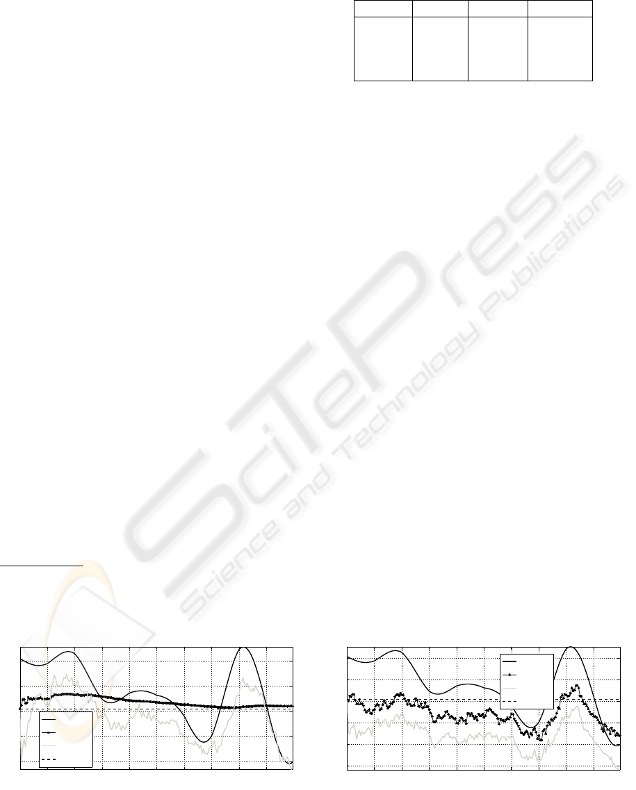
and the EIVjeKf can be explained by regarding the
estimate of b
k
, which is shown in Figure 2. Since the
EIVjeKf models the variations of b
k
by means of Σ
d
,
it is able, to a certain degree, to track b
k
, while the
EIVeKf uses no adaptivity to estimate θ
k
. However,
it would be a straightforward step to include Σ
d
into
the EIVeKf algorithm. In such a case, both estimates
become nearly identical and the corresponding filter
performance (E[P
u
] = 41.8 and E[P
y
] = 48.6) is very
similar to the results of the EIVjeKf (cf. Table 1). The
remaining differences may be explained by the fact
that while the prediction phase of the EIVeKf utilises
the estimates of θ
k
, the default parameter set θ
d
is still
used for the correction.
Another point to be observed in Figure 2 is that
the estimate for b
k
produced by the EIVjeKf is bi-
ased. This was expected, as mentioned in Remark 4.1,
since the parameter estimator resulting from the eKf
approach is not adjusted for the EIV case. Hence, the
EIV filter performance of the nonlinear approaches
can deteriorate if the bias is large with respect to the
model mismatch characterised by θ
d
. In such a situa-
tion, the EIVeKf is expected to perform better than the
EIVjeKf, since the latter relies completely on
ˆ
θ
k
. This
can be verified by modifying the above simulation
and increasing the input noise to Σ
˜u
= 1, which cor-
responds to SNR
u
= −0.1. The filter performance
1
is given in Table 2 and the time-varying parameter b
k
and its estimates are shown in Figure 3. It can be ob-
served, that the estimate produced by the EIVjeKf be-
comes more biased as Σ
˜u
increases resulting in a de-
1
Note, that in this case, Σ
d
is incorporated into the
EIVeKf algorithm.
500 1000 1500 2000 2500 3000 3500 4000 4500
2
3
4
5
6
samples
amplitude
true
EIVeKf
EIVjeKf
default
b
k
Figure 2: Time-varying parameter b
k
, its estimates and the
default value.
Table 2: Filter performance for the different filters for the
case Σ
˜u
= 1.
Kf EIVeKf EIVjeKf
E[P
u
] 39.5 36.1 16.7
E[P
y
] 18.4 24.9 20.0
var(P
u
) 0.8 0.7 3.7
var(P
y
) 0.8 0.8 5.2
creased filter performance, while the estimate given
by the EIVeKf is less biased, hence, by opposition,
yielding a better filter performance.
7 CONCLUSIONS
The solution of the EIV filtering problem as a spe-
cial case of traditional Kalman filtering in extended
noise environments (Diversi et al., 2005) has been re-
viewed. Since the optimal estimation of noise-free
inputs and outputs can be achieved by applying the
well known Kalman filter to a reformulated model, a
joint state and parameter estimation procedure via ex-
tended Kalman filtering (Ljung, 1979) is investigated
for the EIV case. The resulting algorithm is very sim-
ilar to the approach presented in (Vinsonneau et al.,
2005). In fact, these nonlinear EIV filter approaches
attempt to estimate the model parameters by means
of a recursive prediction error method. In turn, this
means that these estimates are generally biased in the
presence of input noise and this may be considered as
the main limitation of these approaches. The differ-
ence between both nonlinear filters is that the EIVeKf
in (Vinsonneau et al., 2005) uses the estimated model
parameters only for the prediction phase of the filter,
and whilst more investigation may be necessary, it ap-
pears to lead to more robustness if the SNR of the in-
put is low.
Some potentially interesting further work would
aim to investigate other suboptimal filters, again with
500 1000 1500 2000 2500 3000 3500 4000 4500
1
2
3
4
5
6
samples
amplitude
true
EIVeKf
EIVjeKf
default
b
k
Figure 3: Time-varying parameter b
k
, its estimates and the
default value for the case Σ
˜u
= 1.
ICINCO 2007 - International Conference on Informatics in Control, Automation and Robotics
52

coupled state and parameter estimation, but where the
parameter set is obtained via a recursive EIV identifi-
cation technique.
REFERENCES
Anderson, B. D. O. and Moore, J. B. (1979). Optimal Fil-
tering. Prentice-Hall, Englewood Cliffs, New Jersey.
Diversi, R., Guidorzi, R., and Soverini, U. (2005). Kalman
filtering in extended noise environments. IEEE Trans.
Autom. Contr., 50:1396–1402.
Guidorzi, R., Diversi, R., and Soverini, U. (2003). Optimal
errors-in-variables filtering. Automatica, 39:281–289.
Ljung, L. (1979). Asymptotic behavior of the extended
Kalman filter as a parameter estimator for linear sys-
tems. IEEE Trans. on Automatic Control, 24(1):36–
50.
Ljung, L. (1999). System Identification - Theory for the
user. PTR Prentice Hall Infromation and System Sci-
ences Series. Prentice Hall, 2nd edition.
Markovsky, I. and De Moor, B. (2005). Linear dynamic
filtering with noisy input and output. Automatica,
41:167–171.
S
¨
oderstr
¨
om, T. (1981). Identification of stochastic lin-
ear systems in presence of input noise. Automatica,
17:713–725.
Vinsonneau, B., Goodall, D. P., and Burnham, K. J. (2005).
Errors-in-variables extended Kalman filter. In Proc.
IAR & ACD Conf., pages 217–222, Mulhouse, France.
AN INVESTIGATION OF EXTENDED KALMAN FILTERING IN THE ERRORS-IN-VARIABLES FRAMEWORK -
A Joint State and Parameter Estimation Approach
53