ESTIMATION OF STATE AND PARAMETERS
OF TRAFFIC SYSTEM
Pavla Pecherkov
´
a, Jitka Homolov
´
a
Dept. of Adaptive Systems, Institute of Information Theory and Automation, Academy of Sciences of the Czech Republic
Pod vod
´
arenskou v
ˇ
e
ˇ
z
´
ı 4, 182 05 Prague 8, Czech Republic
Jind
ˇ
rich Dun
´
ık
Department of Cybernetics, Faculty of Applied Sciences, University of West Bohemia in Pilsen
Univerzitn
´
ı 8, 306 14 Pilsen, Czech Republic
Keywords:
Traffic system, state space model, state estimation, identification, nonlinear filtering.
Abstract:
This paper deals with the problem of traffic flow modelling and state estimation for historical urban areas. The
most important properties of the traffic system are described. Then the model of the traffic system is presented.
The weakness of the model is pointed out and subsequently rectified. Various estimation and identification
techniques, used in the traffic problem, are introduced. The performance of various filters is validated, using
the derived model and synthetic and real data coming from the center of Prague, with respect to filter accuracy
and complexity.
1 INTRODUCTION
Intelligent traffic control is one possible way how
to preserve or to improve capacity of current light
controlled network. Generally, the problem can be
solved by setting proper parameters of the signal
lights. However, the suitable setting of these parame-
ters is conditioned by exact knowledge of the current
traffic situation at an intersection or micro-region
1
.
Nowadays, when many intersection arms are
equipped by detectors
2
, the traffic situation can be
sufficiently described by measurable intensity, occu-
pancy, instant speed and hardly measurable queue
length. Unfortunately, the knowledge of the queue
length seems to be advantageous for a design of traf-
fic control which can be based on the minimisation of
the queue lengths (Kratochv
´
ılov
´
a and Nagy, 2004).
The key problem, either for estimation or control,
is to specify the model of a micro-region. It is very
interesting that the traffic situation can be described
by a linear state space model (SSM) (Homolov
´
a and
Nagy, 2005), where the directly immeasurable queue
lengths are included in the state. Unfortunately, there
1
One micro-region consists of several intersections with
some detectors on the input and output roads. There must
be at least one signal-controlled intersection.
2
Detector is a inductive loop built in a cover of road,
which is activated by a passing vehicle.
are also some unknown parameters in the SSM, which
cannot be determined from physical properties of the
traffic situation and they have to be estimated as well.
Generally, there are two possibilities how to esti-
mate the state and the parameters. The first possibil-
ity is based on an off-line identification of unknown
parameters: prediction error methods (Ljung, 1999),
instrumental variable methods (S
¨
oderstr
¨
om and Sto-
ica, 2002), subspace identification methods (Viberg,
2002)) and subsequently on an on-line estimation of
the state by the well-know Kalman Filter (KF) (An-
derson and Moore, 1979). However, off-line identi-
fied time variant or invariant parameters represent the
average values rather than the actual (true) parame-
ters. The second possibility is based on the concur-
rent on-line estimation of the state and the parameters
by suitable nonlinear estimation methods. There are
two main groups of estimation methods for nonlinear
systems, namely local and global methods (Sorenson,
1974). Although, the global methods are more so-
phisticated than local methods, they have significantly
higher computation demands. Due to the computa-
tional efficiency, the stress will be mainly laid on the
local methods, namely on the local derivative-free fil-
tering methods (Nørgaard et al., 2000; Julier et al.,
2000; Dun
´
ık et al., 2005) and partially will be laid on
a global method based on the Gaussian sums (Dun
´
ık
et al., 2005).
223
Pecherková P., Homolová J. and Duník J. (2007).
ESTIMATION OF STATE AND PARAMETERS OF TRAFFIC SYSTEM.
In Proceedings of the Fourth International Conference on Informatics in Control, Automation and Robotics, pages 223-228
DOI: 10.5220/0001648402230228
Copyright
c
 SciTePress

The aim of this paper is to apply and to compare
the various estimation techniques in the area of the
estimation of queue lengths and parameters of traffic
system and to choose a suitable estimation technique
with respect to the estimation performance and com-
putational demands.
2 TRAFFIC MODEL
2.1 Traffic Model and its Parameters
This paper deals with the estimation of immeasurable
queue length
3
on each lane
4
of controlled intersec-
tions in a micro-region. Lane can be equipped by
one detector on the output and three detectors on the
input: (i) detector on stop line, (ii) outlying detec-
tor, (iii) strategic detector. Ideally, each lane has all
three types of the detectors but in real traffic system,
the lane is usually equipped by one or two types of
such detectors, due to the constrained conditions. The
strategic detectors, which are most remote from a stop
line, give the best information about the traffic flow at
present.
The detector is able to measure following quanti-
ties:
• Intensity I
i,t
is the amount of passing unit vehicles
on arm i per hour [uv/h].
• Occupancy O
i,t
is the proportion of the period
when the detector is occupied by vehicles [%].
Traffic flow can be influenced by signal lights setting.
A signal scheme can be modified by split, cycle time
and offset:
• Cycle time is time required for one complete se-
quence of signal phases [s].
• Split z
t
is proportional duration of the green light
in a single cycle time [%].
• Offset is the difference between the start (or end)
times of green periods at adjacent signals [s].
The geometry of intersections and drivers demands
determine other quantities which are needed for a
construction of the traffic model. These quantities are
valid for a long time period. They are:
• Saturated flow S is the maximal flow rate achieved
by vehicles departing from the queue during the
green period at cycle time [uv/h].
3
Queue length ξ
t
is a number of vehicles waiting to pro-
ceed through an intersection (given in unit vehicles [uv] or
meters [m]) per cycle time. It is supposed that 1 uv = 6 m.
4
Each intersection arm consists of one or more traffic
lanes.
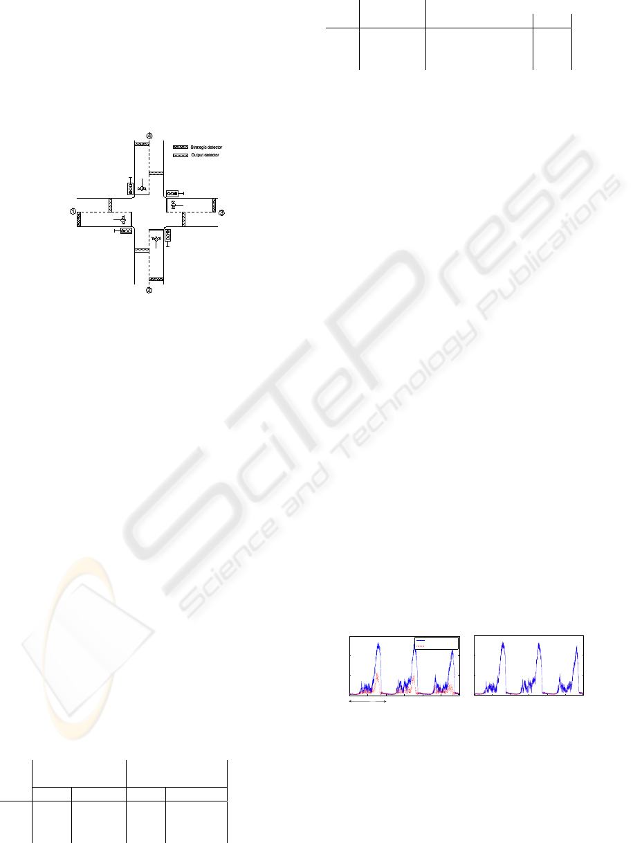
Figure 1: The micro-region: three-arm intersection with
one unmeasured input.
• Turning rate α
h,g
is the ratio of cars going from
the h-th arm to the g-th arm [%].
The basic idea, which lies on the background of
the model design, is the traffic flow conservation prin-
ciple (Homolov
´
a and Nagy, 2005): “the new queue is
equal to the remaining queue plus arrived cars minus
departed cars”.
The basic methodology of the traffic model de-
sign will be shown on a specific example. The micro-
region consists of one three-arm controlled intersec-
tion with one unmeasured input, see Figure 1. Inter-
section is comprised of two one-way input arms (No.1
and 3) and one output arm (No. 2). The input arms
are equipped by the strategic detectors and the output
arm is equipped by the output detector. The unmea-
sured flow enters to the road No. 2 before the output
detector. For the sake of the simplicity, the constant
cycle time with two phases is considered.
In this case, the traffic system is described by
the following model given by (1), (2), where b
i,t
=
(1 − δ
i,t
) · I
i,t
− δ
i,t
S
i
. Parameter δ
i,t
is Kronecker
function (0 , 1), δ
i,t
= 1 if queue exist (on arm i at
time t) and δ
i,t
= 0 in otherwise. Parameters κ
i,t
, ϑ
t
describe the relation between occupancy and queue
length and parameter β
i,t
describes the relation be-
tween current and previous occupancy. The param-
eter λ
i,t
can be understood as a correction term to
omit a zero occupancy. I
i,t
and O
i,t
are the input
intensity and occupancy, respectively, measured by
the input detectors. Y
i,t
is output intensity which is
measured on the output detector. Mention that the
subscript i stand for the number of intersection arm.
The state and measurement noises are currently sup-
posed to be Gaussian, i.e. p(w
k
) =
N {w
k
: 0,Q
k
} and
p(v
k
) =
N {v
k
: 0, R
k
}. The noise covariance matri-
ces Q
k
and R
k
can be identified off-line by means of
e.g. the prediction error method (Ljung, 1999) or the
method based on the multi-step prediction (
ˇ
Simandl
and Dun
´
ık, 2007). On-line noise covariance matrices
estimation, so called adaptive filtering, has not been
used due to the extensive computational demands.
Generally, traffic model can be described in matrix
ICINCO 2007 - International Conference on Informatics in Control, Automation and Robotics
224




ξ
1,t+1
ξ
3,t+1
O
1,t+1
O
3,t+1



|
{z }
x
t+1
=



δ
1,t
0 0 0
0 δ
3,t
0 0
κ
1,t
0 β
1,t
0
0 κ
3,t
ϑ
t
β
3,t



|
{z }
A
t
·x
t
+



−b
1,t
0
0 −b
3,t
0 0
0 0



|
{z }
B
t
·

z
1,t
z
2,t

|
{z }
z
t
+



I
1,t
I
3,t
λ
1,t
λ
3,t



|
{z }
F
t
+w
t
(1)


Y
2,t+1
O
1,t+1
O
3,t+1


|
{z }
y
t+1
=


−α
1,2
−α
3,2
0 0
0 0 1 0
0 0 0 1


|
{z }
C
·x
t+1
+



ξ
1,t
ξ
3,t
0
0



|
{z }
G
t
+v
t+1
(2)
form as follows:
x
t+1
= A
t
x
t
+ B
t
z
t
+ F
t
+ w
t
(3)
y
t+1
= Cx
t+1
+ G
t
+ v
t+1
(4)
The last comment deals with the system ini-
tial condition. The starting time is chosen at early
morning hours, when it can be supposed that there
is no traffic in the micro-region and thus the sys-
tem initial state is perfectly known and it is x
0
=

0 0 0 0

T
.
2.2 Nonlinearities in Traffic Model
The traffic model becomes nonlinear in two main
cases. The first case is when the traffic system has
one or more unmeasured inputs or outputs (and the
particular intensities should be estimated). The sec-
ond case is when the parameters κ
i,t
, β
i,t
, λ
i,t
, and ϑ
t
,
which cannot be determined from the physical proper-
ties and from construction dispositions of the micro-
region, are estimated as a part of the state.
To find an actual estimates of the parameters, it
is necessary to estimate them on-line. One of the
possibilities is to extend the system state with these
parameters ˜x
t
= [x
T
t
,κ
1,t
,κ
3,t
,β
1,t
,β
3,t
,λ
1,t
,λ
3,t
,ϑ
t
]
T
(Anderson and Moore, 1979). This extension in-
evitably also leads to a nonlinear SSM
˜x
t+1
= f
t
( ˜x
t
,z
t
) + w
t
(5)
y
t+1
=
˜
C˜x
t+1
+ G
t
+ v
t+1
(6)
and to an application of appropriate nonlinear estima-
tion techniques. The variables with tildes stand for
the variables which had to be modified due to the ex-
tension of the state.
It should be also mentioned that the concurrent
estimation of the state and parameters is also advan-
tageous for the unusual traffic situations, e.g. acci-
dents, when the estimator adapts the model and the
estimated results are significantly more exact towards
the model with invariant parameters.
3 STATE ESTIMATION
TECHNIQUES
This section is devoted to a brief introduction of pos-
sible estimation methods which can be used for the
estimation of traffic system state. With respect to the
nature of this problem only, a special part of the esti-
mation problem will be considered, namely the filter-
ing.
The aim of the filtering is to find a state estimate
in the form of the probability density function of the
state x
t
at the time instant t conditioned by the mea-
surements y
t
= [y
0
,y
1
,.. .,y
t
] up to the time instant
t, i.e. the conditional pdf p
x
t
|y
t
(x
t
|y
t
) is looked for.
General solution to the filtering problem is given by
the Bayesian Recursive Relations (BRRs) (Anderson
and Moore, 1979).
The exact solution of the BRRs is possible only
for a few special cases, e.g. for linear Gaussian sys-
tem (with known parameters). In other cases, such
as linear system with unknown parameters, nonlinear
and/or non-Gaussian systems, it is necessary to apply
some approximative method, either local or global.
The local methods are often based on approxima-
tion of the nonlinear functions in the state or measure-
ment equation so that the technique of the Kalman Fil-
ter design can be used for the BRRs solution. This ap-
proach causes that all conditional probability density
functions (pdfs) of the state estimate are given by the
first two moments. This rough approximation of pos-
terior estimates induces local validity of the state es-
timates and consequently impossibility to ensure the
convergence of the local filter estimates. The result-
ing estimates of the local filters are suitable mainly
for point estimates. On the other hand, the advantage
of the local methods can be found in the simplicity of
the BRRs solution. Generally, there are two main ap-
proaches in the local filter design. The first possibility
is to approximate the nonlinear function in the model
by means of the Taylor expansion first or second or-
ESTIMATION OF STATE AND PARAMETERS OF TRAFFIC SYSTEM
225

der, which leads e.g. to the Extended Kalman Filter,
or by means of the Stirling’s polynomial interpola-
tion, which leads to the Divided Difference Filter first
or second order, abbreviated as (DD1), (DD2) or to-
gether as (DDFs) (Nørgaard et al., 2000; Dun
´
ık et al.,
2005). The second possibility, often used in the local
filter design, is based on the approximation of state
estimates by a set of deterministically chosen points.
This method is known as the Unscented Transforma-
tion and its application in the local filter design leads
to e.g. the Unscented Kalman Filter (UKF) (Julier
et al., 2000; Dun
´
ık et al., 2005).
The global methods are rather based on approxi-
mation of the conditional pdf of the state estimate of
some kind to accomplish better state estimates.
Due to the higher computational demands of the
global methods, the main stress will be laid on the
local methods especially on the derivative-free local
methods, namely the DD1, the DD2, and the UKF.
The derivative-free methods were chosen because of
there is no need of computations of derivatives of non-
linear functions (Dun
´
ık et al., 2005) which is tedious
especially for high dimensional systems like traffic
systems. However, some attention will be paid on the
Gaussian sum approach as a representative of global
methods. Moreover, the KF with off-line identifica-
tion methods will be considered as well.
4 ANALYSIS OF MODEL
In the previous sections, the model design, estima-
tion and identification techniques were discussed and
it was also mentioned that the quality of the model af-
fects the estimation performance of all filters. From
the more detailed analysis of the traffic model, it is ev-
ident that the estimated state has a backward impact
on the model through the parameter δ
t
. That is the
main weakness of the model because δ
t
depends on
the queue length which is estimated. In other words,
δ
t
can be understood as a parameter which switches
between two models representing peak and off-peak
hours. The problem arises in the situations when the
traffic flow is in the transition from off-peak to peak
hours. Then, δ
t
can be switched from 0 to 1 although
the real traffic flow still corresponds to value 0 and
vice versa, due to non-exact state estimate.
There are two possibilities how to rectify this
problem. The first one is based on the modification
of the state equation(s) describing the evolution of
the queue length (the first two equations in (1)). The
discontinuous equation is approximated by the con-
tinuous approximation based on the hyperbolic tan-
gent, as it is depicted in Figure 2, where the relation
0 10 20 30 40 50 60 70 80 90 100
0
5
10
15
20
25
30
35
40
Queue length
Departed cars
original discontinuous function
aproximation with hyperbolic tangent
Saturation
δ=0
δ=1
Figure 2: The approximation of the discontinuous function
in the state equation.
between queue lengths and number of departed cars
is shown. Then, the continuous approximation pre-
vents from the bad switching of the models. Note that
such approximation is done for all intersection arms.
The second possibility is based on the Gaussian sum
method and on the multi-model approach. It is still
assumed that parameter δ
t
belongs into the discrete
set {0,1} but at each time instant both values are used
and the most probable value is looked for and then
chosen. In case of more arms, all possible combina-
tions of δ
i,t
are tested and the most probable combi-
nation is chosen.
5 NUMERICAL ILLUSTRATIONS
In this section, the different micro-regions, either syn-
thetic or real, will be described and the estimation task
will be performed on each of them.
5.1 Synthetic Micro-regions
Micro-region with short queues: Let a micro-region
consisting of one four-arm controlled intersection be
considered, see Figure 3. All input roads are equipped
by the strategic detectors. For estimation, the data
from real traffic network supplemented with synthetic
data was used. The queue lengths, supposed to be
“true”, and the missing output intensities were deter-
mined with simulation software AIMSUN
5
.
The traffic model was built analogously to the
model (1), (2). The original state has dimension
dim(x
t
) = 8 (queues and occupancies on four arms)
and extended state has dimension dim( ˜x
t
) = 24 (origi-
nal state and unknown parameters κ
i,t
, β
i,t
, λ
i,t
, ϑ
i, j,t
,
i, j = 1,... ,4).
All local filters show very similar estimation per-
formance in the traffic problem. The reason can
be found in a absence from significant nonlinearities
(Dun
´
ık et al., 2005). Thus the results of the DD1 will
be presented only.
5
AIMSUN is a simulation software tool which is able to
reproduce the traffic condition of any traffic network.
ICINCO 2007 - International Conference on Informatics in Control, Automation and Robotics
226

The local filter will be applied on three variants of
model: (A) standard model illustrated by (1), (2), (B)
model with continuous approximation of δ functions,
and (C) multi-model approach. The variant (A) works
with δ as Kronecker function. In the variant (B), the
switching of parameter δ is replaced by the approx-
imation with hyperbolic tangent. In the variant (C),
the model includes Kronecker function δ as well but
switching is replaced by multi-modal approach (by
“brute” force) where the state of models with all com-
binations of δ functions are estimated.
Figure 3: The micro-region: one four-arm controlled inter-
section.
Table 1 shows a comparison of all three variants
with respect to the estimation performance for dif-
ferent types of traffic flows and to the computation
load. The weak traffic flow is characterised by small
intensities and on the other hand working days are
rather characterised by high intensities. The estima-
tion performance is measured by the Mean Square Er-
ror (MSE) of estimates queue length on one arm in
[uv
2
]. The average queue length is about 20 cars in all
arms.
The best estimation performance, with respect to
the MSE, shows the approach (C). On the other hand,
the utilisation of the original model (A) leads to the
least computational demand. With respect to Table
2, where the maximal differences between real and
estimate queue are given, the best approach is multi-
model. The same case is with the number of unsuit-
able values, which are defined as ξ
real
+ 4 < ξ
est
.
For the needs of traffic control, the estimation
method should be sufficiently exact (with small num-
ber of estimates which exceed allowable bound) and
computational efficient. From the results, the best
choice seems to be approach (B) and the DD1.
Table 1: Comparison of the different approaches with re-
spect to the function δ (criterion no. 1).
2 days (weekend) 5 days (workweek)
(1920 samples) (4800 samples)
MSE Time MSE Time
(A) 10.9 26 s 12.5 62 s
(B) 9.4 49 s 7.9 115 s
(C) 8.9 404s 7.1 858 s
Table 2: Comparison of the different approaches with re-
spect to the function δ (criterion no. 2).
Maximal No. of unsuitable values
difference (from 19200 data) [%]
(A) 13.3 3284 17.0
(B) 15.7 1183 6.1
(C) 24.0 1086 5.7
Mention that the KF for micro-region with all
measured arms provides little bit worse but compa-
rable results with local filters and approach (A).
Micro-region with long queues: The typical
micro-region has some arms unequipped by the detec-
tor. This situation together with a long queue lengths
on the access roads will be illustrated in this part.
Let a micro-region consisting of one one-way
three-arm controlled intersection and one unmeasured
input given by (1), (2) be considered, see Figure 1.
The two input roads have strategic detectors and one
output road is equipped by an output detector. More-
over, the long queues on the access road will be con-
sidered to illustrate the situation with permanently en-
gaged detectors which are not able to provide suffi-
cient information about the current traffic flow.
For this simulation, the real data was used but
the intensities were artificially increased. The “true”
queue lengths were computed subsequently by means
of simulation.
The four-dimensional state equation (1) includes
eight a priory unknown parameters (κ
t
, β
t
, λ
t
, ϑ
t
for
each measured input road). All these parameters and
the immeasurable intensity can be estimated by the
local filters. The KF is able to estimate the original
state only and so for the application of the KF, the
model was identified off-line by the prediction error
method (Ljung, 1999) and the unmeasured intensity
was considered as long time average value.
The results of the DD1 were compared with the
KF results. The “true” and estimated queue lengths
of both filters are depicted in Figure 4. It clearly
shows the estimation improvement of the DD1, which
is significantly better and perfectly matches the “true”
queue on arm no. 3 contrary to the KF results.
0 480 960 1440 1920 2400 2880
0
200
400
600
DD1
0 480 960 1440 1920 2400 2880
0
200
400
600
KF
Queue length
on arm no. 3 [m]
real queue
estimated queue
1 day
Figure 4: Comparison of the KF and local filter in the prob-
lem of queue estimation in the micro-region with unmea-
sured input intensity.
5.2 Real Micro-region
For the last experiment, the estimation of queue
lengths was tested on data from the micro-region in
ESTIMATION OF STATE AND PARAMETERS OF TRAFFIC SYSTEM
227

Figure 5: The micro-region: two four-arm controlled and
three uncontrolled intersections.
Prague including two four-arm controlled intersec-
tions and three uncontrolled ones. The arms are one-
way and they consist of several lanes, see Figure 5.
Two input arms are equipped by strategic detectors
and one input arm by outlying detector. Output detec-
tors are in two arms.
For queue estimation, the state space model (3)
and (4) without any approximation was used. The ex-
tended state is dim( ˜x
t
) = 50.
The input and output intensities, occupancies and
green times were measured on the real traffic net dur-
ing several months with sample period 90 sec. The
“true” queue length was again determined with sim-
ulation software AIMSUN. Comparing of the esti-
mated states and simulated ones shows that the esti-
mation depends on the type of input detector. In lanes,
which are equipped by the strategic detector, was usu-
ally MSE ≈ 17, the error is about 10% with respect
to the maximal queues. On the other hand, in lanes,
equipped by the outlying detectors only, the good re-
sults was only in cases where the queue did not exceed
the outlying detector. This is residual queue and for
evaluation of traffic situation is not interesting.
The experiments show that the nonlinear estima-
tion methods are a sufficient tool for estimation of the
queue lengths, even in a real network. The dimension
of the state, which is extended due to the estimation of
parameters or intensities, increases the computation
time, however, the computational demands remains
still feasible (namely the DD1 and model variant (B)).
6 CONCLUSION
The problem of the queue length estimation, which
is hardly measurable quantity, was considered in this
paper. For the queue estimation, the mathematical
model was presented, which describes the micro-
region including its physical properties and taking
into account behaviour of drivers. The disadvan-
tage of the model was highlighted and two possi-
ble solutions of that were proposed. The theoreti-
cal results were illustrated by the numerical examples
based on the synthetic or real data. It was shown that
the Kalman Filter is suitable for situations where all
quantities are measured. In other cases, it is advanta-
geous to use a nonlinear filters for concurrent estima-
tion of the state and parameters or possibly other un-
measurable quantities together with improved model.
ACKNOWLEDGEMENTS
The work was supported by the Ministry of Educa-
tion, Youth and Sports of the Czech Republic, project
No. 1M0572 and by the Ministry of Transport of the
Czech Republic, project No. 1F43A/003/120.
REFERENCES
Anderson, B. D. O. and Moore, S. B. (1979). Optimal Fil-
tering. Englewood Cliffs, New Jersey: Prentice Hall
Ins.
Dun
´
ık, J.,
ˇ
Simandl, M., Straka, O., and Kr
´
al, L. (2005).
Performance analysis of derivative-free filters. In
Proceedings of the 44th IEEE Conference on Deci-
sion and Control, and European Control Conference
ECC’05, pages 1941–1946, Seville, Spain. ISBN: 0-
7803-9568-9, ISSN: 0191-2216.
Homolov
´
a, J. and Nagy, I. (2005). Traffic model of a
microregion. In Preprints of the 16th IFAC World
Congress, pages 1–6, Prague, Czech Republic.
Julier, S. J., Uhlmann, J. K., and Durrant-White, H. F.
(2000). A new method for the nonlinear transforma-
tion of means and covariances in filters and estimators.
IEEE Transactions On AC, 45(3):477–482.
Kratochv
´
ılov
´
a, J. and Nagy, I. (2004). Traffic control of mi-
croregion. In Andr
´
ysek, J., K
´
arn
´
y, M., and Krac
´
ık,
J., editors, CMP’04: Multiple Participant Decision
Making, Theory, algorithms, software and app., pages
161–171, Adelaide. Advanced Knowledge Int.
Ljung, L. (1999). System identification: theory for the user.
UpperSaddle River, NJ: Prentice-Hall.
Nørgaard, M., Poulsen, N. K., and Ravn, O. (2000). New
developments in state estimation for nonlinear sys-
tems. Automatica, 36(11):1627–1638.
S
¨
oderstr
¨
om, T. and Stoica, P. (2002). Instrumental variable
methods for system identification. Circuits, Systems,
and Signal Processing, 21(1):1–9.
Sorenson, H. W. (1974). On the development of practical
nonlinear filters. Inf. Sci., 7:230–270.
Viberg, M. (2002). Subspace-based state-space system
identification. Circuits, Systems, and Signal Process-
ing, 21(1):23–37.
ˇ
Simandl, M. and Dun
´
ık, J. (2007). Multi-step prediction
and its application for estimation of state and mea-
surement noise covariance matrices. Technical report.
University of West Bohemia in Pilsen, Department of
Cybernetics.
ICINCO 2007 - International Conference on Informatics in Control, Automation and Robotics
228