
FORWARD KINEMATICS AND GEOMETRIC CONTROL OF A
MEDICAL ROBOT
Application to Dental Implantation
Richard Chaumont, Eric Vasselin and Dimitri Lefebvre
GREAH of LE HAVRE University, 25 rue Philippe LEBON. 76058 LE HAVRE Cede, France
Keywords: Surgical robotics, geometric modelling, inverse geometric modelling, dynamic modelling, non linear
system, identification.
Abstract: Recently, robotics has found a new field of research in surgery in which it is used as an assistant of the
surgeon in order to promote less traumatic surgery and minimal incision of soft tissue. In accordance with
the requirements of dental surgeons, we offer a robotic system dedicated to dental implants. A dental
implant is a mechanical device fixed into the patient’s jaw. It is used to replace a single tooth or a set of
missing teeth. Fitting the implant is a difficult operation that requires great accuracy. This work concerns
the prototype of a medical robot. Forward and inverse kinematics as dynamics are considered in order to
drive a control algorithm which is as accurate and safe as possible.
1 INTRODUCTION
Computer-assisted dental implantology is a
multidisciplinary and complex topic that includes
medical imagery, robotics and computer vision
(Langlotz, & al, 2000 ; Nikou & al, 2000). The
fitting of a dental implant is currently the only
technique suitable to permanently restore the teeth.
For this purpose, specific surgery has been recently
developed. Such operations require great accuracy.
Moreover, the spread of this type of surgery justifies
the extension and use of new techniques (Taylor,
1994). This research and development work focuses
on the medical robotics applied to dental
implantology. The main contributions of this article
are to discuss the forward kinematics and kinematics
uncertainties, and also to provide a geometric
control for the orientation of the drill.
2 MEDICAL ROBOTICS
For the last twenty years, new technologies have
been used to improve surgical operations so that
medical research and engineering improvements are
closely linked today. On one hand, data processing,
computer vision and medical imaging are used in an
intensive way in operation rooms. On the other
hand, the three principles of robotics-perception,
reasoning and action - have been adapted for
medical and surgery issues (Lavallee & al, 1995).
The main goal is to bring together the fundamental
principles of robotics and computer vision in order
to assist the surgeon in daily therapeutic operations.
The aims of medical robotics are to provide less
traumatic investigation systems, to provide
simulation tools, and, finally, to provide tools that
are easier and more flexible to use.
The aim of dental implantology is to use bones
and implants in order to provide prosthetic support.
The main advantage in comparison with a
conventional prosthesis is that dental implantology
doesn't mutilate healthy teeth. At the time tooth
extraction is completed, the fitting of a dental
implant allows the consolidation of the prostheses.
The main difficulty is to place the implants
correctly. That is the reason why conventional
prosthesis is still prefered to dental implantology in
many cases.
Dental implants guarantee the patient better
comfort but can also reduce overall cost owing to
their longevity and lack of inherent complications in
comparison with classic prostheses. For difficult
cases (completely toothless patients, weak density
bones, multiple implants, etc), dental surgeons are
confronted with a complex operation. Over the
years, the main difficulty concerned the integration
of the bone-implant.
This problem has been solved by technical
improvements and surgical advances (equipment,
implant shapes, surgical protocol, etc). According to
110
Chaumont R., Vasselin E. and Lefebvre D. (2007).
FORWARD KINEMATICS AND GEOMETRIC CONTROL OF A MEDICAL ROBOT - Application to Dental Implantation.
In Proceedings of the Fourth International Conference on Informatics in Control, Automation and Robotics, pages 110-115
DOI: 10.5220/0001652501100115
Copyright
c
SciTePress
the opinion of many clinicians, the difficulty is
henceforth to improve fitting techniques. The
position and orientation of implants must take into
account biomechanical and anatomical constraints
(Dutreuil, 2001) involving three main criteria:
mastication, phonetics and aesthetics. In particular,
the problems to be solved are :
• How to adjust the implant position in the
correct axis.
• How to optimize the relative position of
two adjacent implants.
• How to optimize the implant position
according to the bone density.
• How to conduct minimal incision of soft
tissue.
Our answer to these questions is image guided
surgery (Etienne & al, 2000). This solution uses an
optical navigation system with absolute positioning
in order to obtain position and orientation of the
surgeon's tool in real time with respect to the
patient’s movements. The operation is planned on
the basis of scanner data or x-ray images for simple
clinical cases.
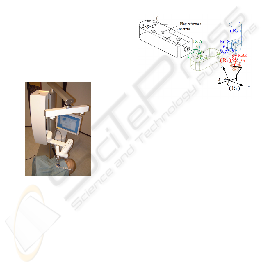
Figure 1: Navigation system.
The technique consists in initializing the
superimposing of patient data and data derived form
a set of specific points attached to the patient’s jaw
(Granger, 2003). The patient’s jaw is then analyzed
in real time by the navigation system. The Dental
View navigation machine guides the surgeon via the
image during the operative phase.
However, clinical tests show that supplementary
assistance is necessary to help the surgeon during
the drilling phase in order to fulfil precision
requirements. For this purpose, we developed a
surgical robot which controls orientation during the
drilling phase.
Our robot is a semi-active mechanical device. It
has a passive arm and a motorized wrist with three
degrees of freedom (dof) that are not convergent (i.e.
not a spherical wrist). The basis is passive, that is to
say it is not motorized and can be manipulated by
the surgeon like an instrument. The aim of the
controller is to guide the surgeon so that it will
respect the scheduled orientation.
3 FORWARD KINEMATICS
Drill orientation is characterized by 3 dof RotY,
RotX and RotZ and depends also on contra angle ca
(Fig. 3). The structure is represented in Fig.2.
Figure 2: Robot axis.
3.1 Notations
We use homogeneous transformations to describe
position and orientation from one link to another.
Let us consider the matrix M :
R
T
M
PQ
⎡
⎤
=
⎢
⎥
⎣
⎦
(1)
with P = [0 0 0], Q = [1] is a homothetic coefficient
equal to 1 (orthogonal transformation); R is a
orthogonal rotation matrix; and T is a translation
matrix.
For simplicity, calculations are not given in
detail. Notations will be represented above Fig.3.
Lxo, Lyo, Lzo : distance x, y, z between computer
vision coordinate frame and 4
th
joint coordinate
frame.
Lx5, Lz6 : distance x, z between 4
th
joint and 5
th
joint.
Lyca, Lzca : distance y, z between 5
th
joint and
effector.
Lztool : drill length.
θ
4
, θ
5
, θ
6
: wrist joint variables.
Ca: contra angle.
ε
i
: orthogonal uncertainty between joints.
l
i
: length uncertainty between links.
FORWARD KINEMATICS AND GEOMETRIC CONTROL OF A MEDICAL ROBOT - Application to Dental
Implantation
111
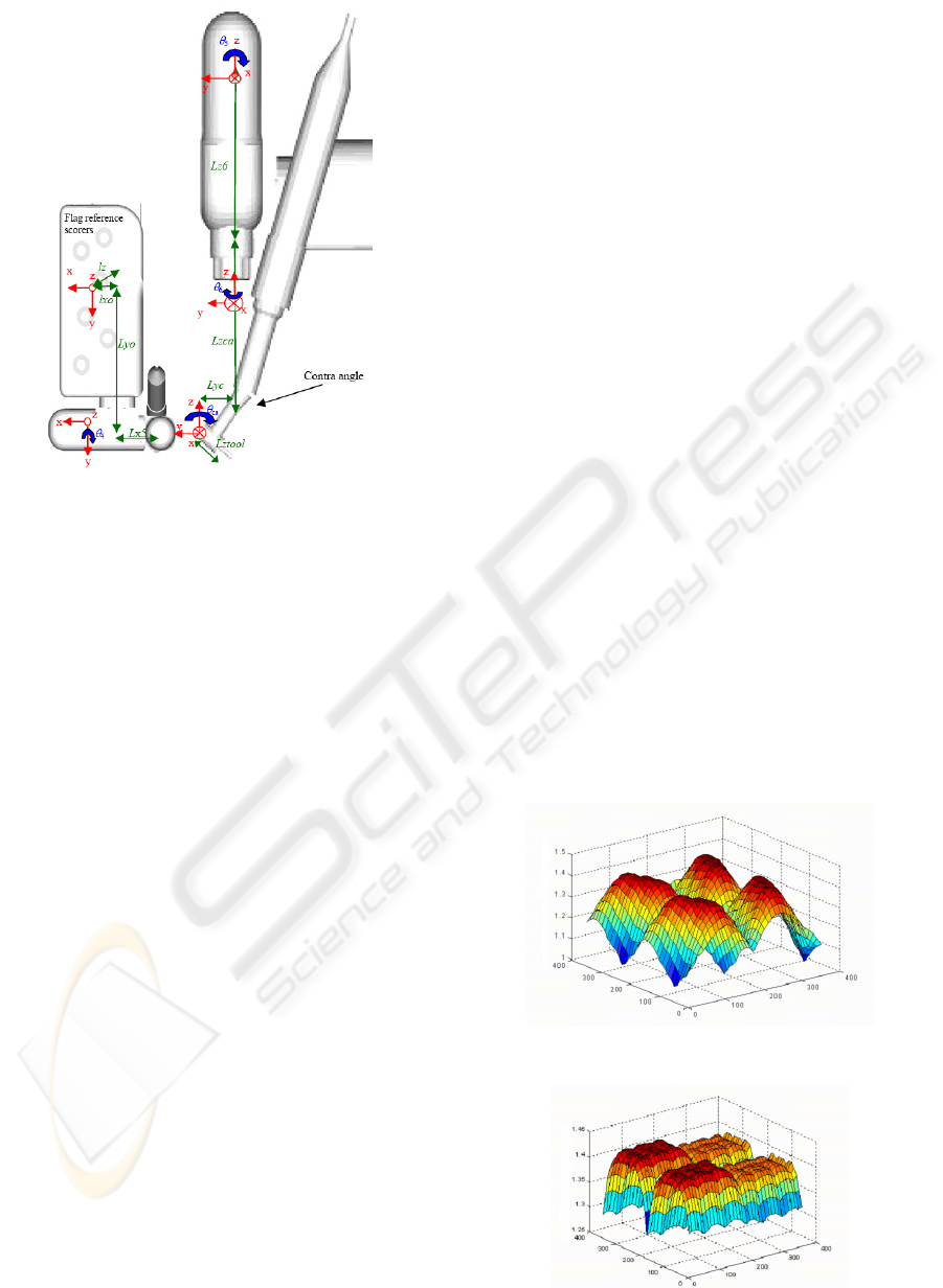
Figure 3: Robot parameters and axes.
3.2 Kinematic Uncertainties
First, we are going to determine the effector position
in the ideal case, without considering uncertainties
related to length and orthogonality links. We use
homogeneous transformations to change the
coordinate frame attached to a joint to the coordinate
frame attached to the next one. We obtain 6 matrices
that change the coordinate frames according to (2) :
100
010
1
001
000 1
Lxo
Lyo
A
Lzo
⎛⎞
⎜⎟
⎜⎟
=
⎜⎟
⎜⎟
⎝⎠
cos 0 sin 0
44
0100
2
sin 0 cos 0
44
0001
A
θθ
θθ
⎛⎞
⎜⎟
⎜⎟
=
⎜⎟
−
⎜⎟
⎝⎠
10 0 5
0cos sin 0
55
3
0sin cos 0
55
00 0 1
Lx
A
θθ
θθ
⎛
⎞
⎜
⎟
−
⎜
⎟
=
⎜
⎟
⎜
⎟
⎝
⎠
cos si n 0 0
66
sin cos 0 0
66
4
0016
0001
A
Lz
θθ
θθ
−
⎛
⎞
⎜
⎟
⎜
⎟
=
⎜
⎟
⎜
⎟
⎝
⎠
10 0 0
0 c os( ) si n( ) 0
5
0sin() cos() 0
00 0 1
ca ca
A
ca ca
⎛
⎞
⎜
⎟
−
⎜
⎟
=
⎜
⎟
⎜
⎟
⎝
⎠
100 0
010
6
001
000 1
Lyca
A
Lzca
⎛⎞
⎜⎟
⎜⎟
=
⎜⎟
⎜⎟
⎝⎠
(2)
Ideal position in flag coordinate frame results
from the preceding matrices :
0 123456 4
() ()
ideal
VRAAAAAAVR=××××××
(3)
with V(R
4
) = [0 0 1 0]
T
to get effector orientation for
the “z” axis and V(R
4
) = [0 0 0 1]
T
to get effector
position.
⎟
⎟
⎟
⎟
⎟
⎠
⎞
⎜
⎜
⎜
⎜
⎜
⎝
⎛
±
±
±
=
1000
100
010
001
'
1
zo
yo
xo
lLzo
lLyo
lLxo
A
10 0 0cos 0sin0cos sin 00
44 22
0 cos sin 0 0 1 0 0 sin cos 0 0
11 22
'
2
0sin cos 0 sin 0cos 0 0 0 10
11 4 4
00 0 1 0001 0 0 01
A
θθ εε
εε εε
εε θ θ
±−±
⎛⎞⎛⎞⎛ ⎞
⎜⎟⎜⎟⎜ ⎟
±−± ± ±
⎜⎟⎜⎟⎜ ⎟
=××
⎜⎟⎜⎟⎜ ⎟
±± −
⎜⎟⎜⎟⎜ ⎟
⎝⎠⎝⎠⎝ ⎠
1 0 0 5 cos 0 sin 0 cos sin 0 0
53 3 44
0 cos sin 0 0 1 0 0 sin cos 0 0
55 4 4
'
3
0 sin cos 0 sin 0 cos 0 0 0 1 0
55 3 3
00 0 1 0 0 0 1 0 0 01
Lx l
x
A
εε εε
θθ ε ε
θθ ε ε
±± ± ±−±
⎛⎞⎛⎞⎛⎞
⎜⎟⎜⎟⎜⎟
−±±
⎜⎟⎜⎟⎜⎟
=××
⎜⎟⎜⎟⎜⎟
−± ±
⎜⎟⎜⎟⎜⎟
⎝⎠⎝⎠⎝⎠
10 0 0cos 0sin 0cos sin0 0
6666
0cos sin 0 0100sincos00
55 66
'
4
0 sin cos 0 sin 0 cos 0 0 0 1 6
55 6 6 6
00 0 1 0 001 0 00 1
A
Lz l
z
εεθθ
εε θθ
εε ε ε
±± −
⎛⎞⎛⎞⎛ ⎞
⎜⎟⎜⎟⎜ ⎟
±−±
⎜⎟⎜⎟⎜ ⎟
=××
⎜⎟⎜⎟⎜ ⎟
±± −± ± ±
⎜⎟⎜⎟⎜ ⎟
⎝⎠⎝⎠⎝ ⎠
100 0
010
'
5
001
000 1
Lyca l
yca
A
Lzca l
z
ca
⎛⎞
⎜⎟
±
⎜⎟
=
⎜⎟
±
⎜⎟
⎜⎟
⎝⎠
1 0 0 0 cos 0 sin 0 cos sin 0 0
55 66
0 cos( ) sin( ) 0 0 1 0 0 sin cos 0 0
'
66
6
0sin() cos() 0 sin 0cos 0 0 0 10
55
00 01 0001 0 001
ca ca
A
ca ca
εε εε
εε
εε
⎛⎞⎛⎞⎛⎞
±± ±−±
⎜⎟⎜⎟⎜⎟
−±±
⎜⎟⎜⎟⎜⎟
=××
⎜⎟⎜⎟⎜⎟
−± ±
⎜⎟⎜⎟⎜⎟
⎜⎟⎜⎟⎜⎟
⎝⎠⎝⎠⎝⎠
(4)
We will model actual position and orientation of
the effector by considering uncertainties relating to
link length (maximum tolerance of 0.1 mm) and also
of frame orthogonal uncertainties (maximum
tolerance 0.1 degree). Because of digital encoder
resolution (200 000 points per revolution) and of
gear reduction encoders uncertainties are negligible.
Moreover, we only consider uncertainties that
concern the robot wrist (the arm is a passive
mechanical structure). For every dof two uncertainty
matrices are added according to the axes that are not
articulated. Equation (4) is obtained as a
consequence.
Actual effector position is given by (5):
0 123456 4
() ' ' ' ' ' ' ()
actual
VRAAAAAAVR
=
××××××
(5)
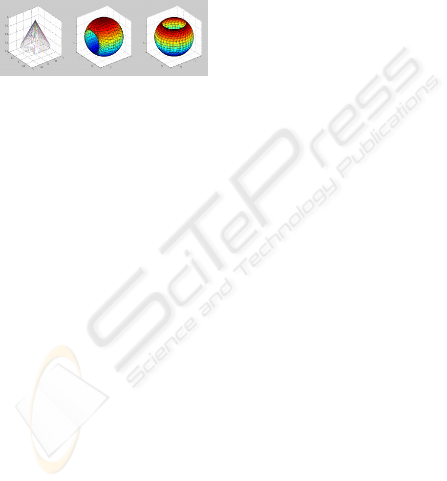
Figure 4: Magnitude of error function for θ
4
and θ
5
.
Figure 5: Magnitude of error function for θ
4
and θ
6
.
ICINCO 2007 - International Conference on Informatics in Control, Automation and Robotics
112
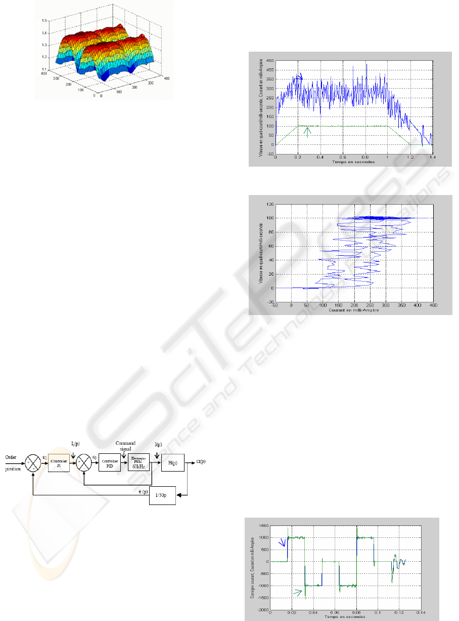
Figure 6: Magnitude of error function for θ
5
and θ
6
.
From (4) and (5), we know the ideal position and
orientation of the wrist as well as its actual position
and orientation which take kinematic uncertainties
into account. Therefore, we can obtain the position
and orientation errors :
000
() () ()
actual ideal
E
RV RV R=−
(6)
Figs. 4 to 6 represent the maximal uncertainty
magnitude (millimeter) generated by mechanical and
assembly tolerances. One observes that :
• Uncertainty magnitude is always superior
to 1 millimeter,
• Uncertainty magnitude can reach 1.4
millimeters for particular link positions.
In order to fulfil precision requirements
uncertainties must be lower than 1 millimeter.
Therefore, it is necessary to calibrate the robot wrist.
4 DYNAMICS
In this section we will propose a dynamic model for
the axis of the robot. The axis control architecture is
presented in Fig.7. Technical caracteristics of the
electromechanical and electronic devices can be
found in (Chaumont & al, 2006).
Figure 7: Axis control structure.
4.1 Identification of Electromechanical
Device
Closed loop identification for electromechanical
device is proposed in this section (Richalet, 1998).
System output is the velocity and system input is the
current. The robot axis has been placed so that
inertia moment can be considered as constant
whatever the orientation.
The time response (Fig. 8) presents a
dissymmetry between the current generating the
acceleration in comparison with the current
generating the deceleration.
Figure 8: Protocol signature.
Figure 9: Hysteresis system.
The process is non linear. Fig. 9 represents
input/output signature with a dead zone and a
histereses. The electromechanical transfer function
is represented in Fig.13.
4.2 Identification of Electronic Device
Electronic device input is the desired current and
output is the actual current. It represents the
electronic system part that is composed of the PWM
and its controller.
Identification is achieved in closed loop. A
survey of electronic control shows us that the
transfer function is a second order overshoot with a
stable zero.
Figure 10: Protocol signature.
Courant
(
mA
)
Speed (quarter-count/ms)
Consi
g
nes en courant
(
mA
)
Courant (mA)
FORWARD KINEMATICS AND GEOMETRIC CONTROL OF A MEDICAL ROBOT - Application to Dental
Implantation
113
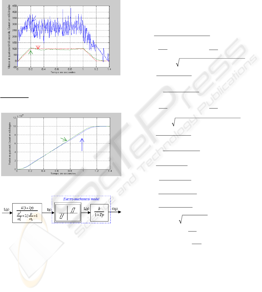
4.3 Discussion
The model is validated with the same desired
current. Results obtained with the model and with
the system are compared according to velocity
kinetics (Fig. 11) and position (Fig. 12).
Figure 11: Velocity response.
Parameters
ω
0
= 730.97; ξ = 0.4258; K = 0.9955; k = 0.5969 ; T = 0.539
Histereses size: 75 mA Dead zone size: 115 mA.
Figure 12: Position response.
Figure 13: Axis module.
5 CONTROL DESIGN
Forward kinematics is given by equation (2). This
model shows how to determine the effector’s
position and orientation in terms of the joint
variables with a function “f”. Inverse kinematics is
concerned with the problem of finding the joint
variables in terms of effector’s position and
orientation. Our aim is to control the orientation of
the effector. The function “f” corresponds therefore
to V
ideal
(R
0
) expressed by equation (3) with V(R
4
) =
[0 0 1 0]
T
(uncertainties are not considered for
control design).
Matrix V
ideal
(R
0
) leads to equations (7) to (9) :
Vx
0
=sin(ca).cos(θ
4
).sin(θ
6
)–sin(ca).sin(θ
4
).
sin(θ
5
).cos(θ
6
)+sin(θ
4
).cos(θ
5
).cos(ca) (7)
Vy
0
= – cos(θ
5
).cos(θ
6
).sin(ca) – sin(θ
5
).cos(ca) (8)
Vz
0
= –sin(ca).sin(θ
4
).sin(θ
6
) –.cos(θ
4
).sin(θ
5
).
cos(θ
6
) + cos(θ
4
).cos(θ
5
).cos(ca) (9)
From equations (7), (8) and (9), expressions θ
4
,
θ
5
and θ
6
are determined.
)sin(
).sin().cos(
asin
0404
6
ca
VzVx
θ
θ
θ
−
=
,
66
θ
π
θ
−=
a
(10)
1
0
5
1
acos a
yV
+
⎟
⎠
⎞
⎜
⎝
⎛
=
ρ
θ
,
1
0
5 .2acos
1
a
yV
a +
⎟
⎠
⎞
⎜
⎝
⎛
−=
ρ
θ
(11)
with :
()
)(cos)sin().cos(
2
2
61
caca +=
θρ
π
θ
+
⎟
⎠
⎞
⎜
⎝
⎛
=
)sin().cos(
)cos(
atan
6
1
ca
ca
a
if -cos(θ
6
).sin(ca) < 0
or
⎟
⎠
⎞
⎜
⎝
⎛
=
)sin().cos(
)cos(
atan
6
1
ca
ca
a
θ
if -cos(θ
6
).sin(ca) > 0
2
2
0
5
acos a
yV
b +
⎟
⎠
⎞
⎜
⎝
⎛
=
ρ
θ
,
2
2
0
5 .2acos a
yV
c +
⎟
⎠
⎞
⎜
⎝
⎛
−=
ρ
θ
(12)
with :
()
)(cos)sin().cos(
2
2
62
caca
a
+=
θρ
π
θ
+
⎟
⎠
⎞
⎜
⎝
⎛
=
)sin().cos(
)cos(
atan
6
2
ca
ca
a
a
if -cos(θ
6a
).sin(ca) < 0
or
⎟
⎠
⎞
⎜
⎝
⎛
=
)sin().cos(
)cos(
atan
6
2
ca
ca
a
a
θ
if -cos(θ
6a
).sin(ca) >0
b
ca
+=
σ
θ
θ
)sin().sin(
acos
6
4
b
ca
aa .2
)sin().sin(
cos
6
4
+−=
σ
θ
θ
b
ca
a
a
b
+=
σ
θ
θ
)sin().sin(
cos
6
4
b
ca
a
a
c
.2
)sin().sin(
cos
6
4
+−=
σ
θ
θ
(13)
with :
2
0
2
0
VzVx +=
σ
(
)
π
−−=
0
0
atan
Vx
Vz
b
if Vx
0
< 0
(
)
0
0
atan
Vx
Vz
b −=
if Vx
0
> 0
Equations (10) to (13) show that angle θ
6
depends on
θ
4
, that angles θ
4
and θ
5
depend on θ
6
. A robot is
"resolvable" if a unique solution exists for equation
θ = f
-1
(x). Our study suggest that our medical
robot’s wrist is not resolvable.
5.1 Reachable Workspace
Analysis of the resulting equations shows that the
determination of the desired current according to a
given set of joint variables θ
4
, θ
5
and θ
6
is difficult.
Courant order (mA)
Process speed (quarter-count/ms)
Model speed (quarter-count/ms)
Position(quater-count)
Consigne position (quater-count)
ICINCO 2007 - International Conference on Informatics in Control, Automation and Robotics
114
Indeed, a given orientation has several solutions for
joint variables. Fig. 14 illustrates these points by
defining the reachable workspace. The method we
propose consists in considering θ
4
as a constant
parameter in order to work out joint variables θ
5
and
θ
6
according to θ
4
. The choice of θ
4
is motivated by
optimization method.
Figure 14: Reachable workspace.
5.2 Control Strategy
The controller must satisfy real time requirements.
The sampling frequency is 20 Hz. Moreover, several
applications such as artificial vision and data
processing take place simultaneously. The controller
inputs are :
• Data from artificial vision and image
superimposition,
• Desired drill orientation,
• Actual angular values returned by digital
encoders.
The algorithm determines the values of V
xo
, V
yo
,
and V
zo
that are vector components in the flag
reference scorers of the robot. It determines θ
5
and
θ
6
with respect to θ
4
and verifies that solutions are in
the reachable workspace. If solutions are outside the
reachable workspace, the algorithm increments θ
4
with 1° and recalculates θ
5
and θ
6
. Incrementation is
repeated until a solution is found in the reachable
workspace.
6 FURTHER WORKS
The protocol used for identification will be applied
in a generic way on the other axes in order to obtain
a dynamic model of the robot. As a consequence, we
will be able to simulate the robot’s dynamic
behaviour and to develop safe and efficient control
design. On the other hand, our work will concern the
following points :
• Accuracy, wrist calibration,
• Study of position / orientation decoupling,
• Trajectory planning, ergonomics.
This medical robot is an invasive and semi-active
system. Therefore, an exhaustive study on reliability
will also be necessary (Dombre, 2001) before
starting clinical simulations and experimentations.
ACKNOWLEDGEMENTS
Authors thank the Doctor DERYCKE, a dental
surgeon specialized in implantology, CHIEF
EXECUTIVE OFFICER of DENTAL VIEW.
REFERENCES
Langlotz F, Berlemann U, Ganz R, Nolte LP., 2000.
Computer-Assisted Periacetabular Osteotomy. Oper.
Techniques in Orthop, vol 10, N° 1, pp. 14-19
Nikou C, Di Gioia A, Blackwell M, Jaramaz B, Kanade
T., 2000. Augmented Reality Imaging Technology for
Orthopaedic Surgery. Oper. Techniques in Orthop, vol
10, N° 1, pp. 82-86.
Taylor R.,1994. An Image Directed Robotic System for
Precise Orthopaedic Surgery. IEEE Trans Robot, 10,
pp. 261-275.
Lavallee S, Sautot P, Traccaz J, P. Cinquin P, Merloz P.,
1995. Computer Assisted Spine Surgery : a technique
for accurate transpedicular screw fixation using CT
data and a 3D optical localizer. Journal of Image
Guided Surgery.
Dutreuil J., 2001. Modélisation 3D et robotique médicale
pour la chirurgie. Thèse, Ecole des Mines de Paris.
Etienne D, Stankoff A, Pennnec X, Granger S, Lacan A,
Derycke R., 2000. A new approach for dental implant
aided surgery. The 4
th
Congresso Panamericano de
Periodontologia, Santiago, Chili.
Granger S., 2003. Une approche statistique multi-échelle
au recalage rigide de surfaces : Application à
l’implantologie dentaire. Thèse, Ecole des Mines de
Paris.
Chaumont R, Vasselin E, Gorka M, Lefebvre D., 2005.
Robot médical pour l’implantologie dentaire :
identification d’un axe, JNRR05. Guidel, pp 304-305.
Richalet J., 1998. Pratique de l’identification. Ed. Hermes.
Dombre E., 2001. Intrinsically safe active robotic systems
for medical applications. 1st IARP/IEEE-RAS Joint
Workshop on Technical Challenge for Dependable
Robots in Human Environments, Seoul, Korea.
A
B
C
FORWARD KINEMATICS AND GEOMETRIC CONTROL OF A MEDICAL ROBOT - Application to Dental
Implantation
115
