VECTOR QUANTISATION BASED IMAGE ENHANCEMENT

W. Paul Cockshott, Sumitha L. Balasuriya, Irwan Prasetya Gunawan and J. Paul Siebert

University of Glasgow, Computing Science Department

17 Lilybank Gardens, Glasgow G12 8QQ, UK

Keywords: Image rescaling, bspline, vector quantization, fractal.

Abstract: We present a new algorithm for rescaling images inspired by fractal coding. It uses a statistical model of the

relationship between detail at different scales of the image to interpolate detail at one octave above the highest

spatial frequency in the original image. We compare it with Bspline and bilinear interpolation techniques and

show that it yields a sharper looking rescaled image.

1 INTRODUCTION

Digital cinema sequences can be captured at a number

of differentresolutions, for example 2K pixels accross

or 4K pixels accross. The cameras used for high res-

olutions are expensive and the data ﬁles they produce

are large. Because of this, studios may chose to cap-

ture some sequences at lower resolution and others at

high resolution. The different resolution sequences

are later merged during post production. The merger

requires that some form of image expansion be per-

formed on the lower resolution sequences. In this pa-

per we present a new method for doing the image ex-

pansion that has some advantages over the orthodox

bilinear or bicubic interpolation methods.

1.1 Traditional Approach

If you scale up a 2K pixel image A to a new image

B which is 4K pixels accross, each original pixel is

being replaced with 4 pixels. But you have no ad-

ditional information as to what these 4 pixels should

contain. If you scale up by interpolation, then the new

pixels in B are generated by some polynomial func-

tion over the corresponding the neighbourhood in the

smaller input image A. A consequence of this is that

the scaled up image looks smoother and contains less

energy at the highest spatial frequencies than the orig-

inal from which it was derived. When one scales up,

one creates new higher spatial frequency bands with

no information as to what they should contain.

1.2 Fractal Enhancement

An alternative approach, fractal encoding, originally

reported by Barnsley(Barnsley and Hurd, 1993), al-

lows rescaled images to contain new high frequency

information. Fractal encoding takes advantage of the

self similarity across scales of natural scenes. A frac-

tal code for an image consists of a set of contractive

afﬁne maps from the image, onto the image. Taken as

a whole, these maps compose a collage such that each

pixel is mapped onto by at least one such map. The

maps operate both in the spatial and the luminance do-

main. In the luminance domain they specify a target

pixel p by an equation of the form p = a + bq where

q is the mean brightness of a downsample region of

source pixels. In the spatial domain they specify the

coordinates of the source pixels supporting q as the

result of rotation, scaling and translation operations

on the coordinates of the destination pixels.

The image is regenerated from the codes by it-

erated application of the afﬁne maps. The iteration

process has an attractor that is the output image. If

the maps have been well chosen this attractor approx-

imates well to a chosen input image.

A particular fractal code might specify each 4x4

rectangle within a 256x256 pixel output image in

terms of a contractive map on some 8x8 rectangle at

some other point in the image. As the iteration pro-

Paul Cockshott W., L. Balasuriya S., Prasetya Gunawan I. and Paul Siebert J. (2007).

VECTOR QUANTISATION BASED IMAGE ENHANCEMENT.

In Proceedings of the Second International Conference on Computer Vision Theory and Applications - IFP/IA, pages 79-84

 SciTePress

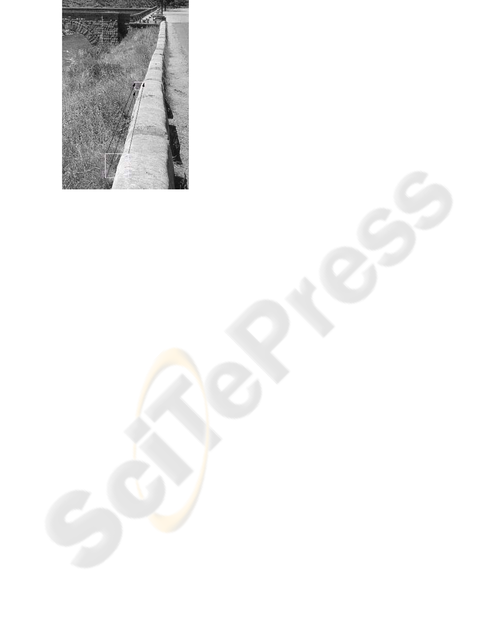
Figure 1: Illustration of how shrinking is used to ﬁll in detail

in fractal enhancement.

ceeds higher and higher frequency information is built

up. If we start from a uniform grey image, the ﬁrst it-

eration will generate detail at a spatial frequency of

8 pixels. After one iteration source blocks of 8 pix-

els accross will contain up to one spatial wave. After

the second interpolation these waves will have been

shifted up in frequency to 4 pixels accross. Each iter-

ation adds detail one octave higher until the Nyquist

limit of the output image is reached: 128 spatial cy-

cles in this case.

It is evident that if we specify the contractivemap-

pings relative to the scale of the whole image rather

than in terms of pixels, then the same set of mappings

could be used to generate a 512x512 pixel output

image. In this case the contractive mappings would

shrink 16 pixel blocks to 8 pixel blocks. After an an

additional round of iteration the 512 pixel output im-

age will contain spatial frequencies up to 256 cycles.

Fractal codes can thus be used to expand an im-

age, generating new and higher spatial frequencies

in the process. Although the additional detail that is

added by this process can not have been available in

the source image it nevertheless ’looks plausible’ be-

cause the ’new’ details are scaled down versions of

details that were present in the original picture ( see

Figure 1). The search process used in a fractal en-

coder scans a half sized copy of the original image

to ﬁnd a match for each small block in the original

image. In fractal enhancement the small blocks are

then replaced by their full sized correspondingblocks.

The detail enhancement comes because there is a sys-

tematic relationship between the low frequency and

high frequency information within blocks. This al-

lows high frequency information in a larger block to

be plausibly substituted into a smaller block when that

is enlarged.

Fractal codes however suffer from two serious ob-

stacles to their widespread adoption: the encoding al-

gorithm is slow and their general use is blocked by

patent restrictions. In this paper we present an alterna-

tive approach that learns lessons from fractal coding

but avoids these difﬁculties. Instead of using fractals

we use vector quantisation to enhance the detail of an

image.

2 OUR ALGORITHM

The key idea of our approach is that because there

is a systematic relationship between low and high fre-

quency information within a neighbourhood,it should

be possible for a machine learning algorithm to dis-

cover what this relationship is and exploit this knowl-

edge when enhancing an image. We use vector quan-

tisation to categorise areas of the image at different

scales, learn the systematic relationship between the

coding of corresponding areas at varying scales, and

then use this information to extrapolate a more de-

tailed image. The entire process works by

1. Running a training algorithm to learn the cross-

scale structure relations in example pictures. In

the experiments here two images were used one

from the ‘face’ sequence and one from the ‘trees’

sequence.

2. Using this information to automatically construct

a new image enhancing program.

3. Applying the enhancing program to digital cine

images to generate new images at twice the reso-

lution.

2.1 The Training Algorithm

The aim of the training algorithm is to learn what high

frequencydetail is likely to be associated with the low

frequencyfeatures at a given point in an image. Given

an image I we construct a half sized version of the im-

age I

0.5

and expand this to form a new blurred image

which is the original size, by using linear interpo-

lation. We now form a difference image I

= I − I

which contains only the high frequency details.

It it clear that we have a genetive association

between position I

0.5

[x, y] and the four pixel block

x,y

= {I

[2x, 2y], I

[2x+ 1,2y], I

[2x, 2y+ 1], I

[2x+

1, 2y + 1]}. We aim to categorise the regions around

each position in I

0.5

[x, y] , categorise the correspond-

ing blocks G

x,y

and learn the associations between

these categories.

2.1.1 Categorising the Upper Layer

Associate with each pixel p ∈ I

0.5

a neighbourhood

and compute the differences between p and its

neighbours. These deﬁne a 4 element vector. Using

the algorithm given in (Linde et al., 1980) construct

a vector quantisation codebook B

for these features.

Assume that the code book has n entries.

2.1.2 Categorising the Lower Layer

Use the same vector quantisation algorithm to con-

struct a second vector quantisation codebook B

for

the set of vectors G

x,y

. Assume that the code book

again has n entries.

2.1.3 Learning the Association

Encode the neighbourhoodsaround each pixel p ∈ I

0.5

with B

to yield an encoded image E

0.5

. Encode each

x,y

associated with each pixel p ∈ I

0.5

with B

yield an encoded image E

. The entries in both the

encoded images are indexes into the respective code-

books.

Construct a n × n frequency table F that counts

how frequently each code from B

is associated with

each code from B

. Finally convert the frequency ta-

ble to a conditional probability table by dividing by

the number of observations.

2.2 The Program Generator

The aim of the program generator is to take the tables

, B

, F and use them to generate pascal libraries

that can be used to index and predict detail in sub-

sequent images. The process is analogous to the way

Lex(Levine et al., 1992) constructs scanner tables in

C from a regular grammar.

Two optimisations are performed prior to output-

ing the tables:

1. Table F is converted from a conditional probabil-

ity table to a table encoding the cumulative prob-

ability of each entry in B

being associated with

and entry in B

2. Hierarchical Vector Quantisation (Chaddha et al.,

1995) indices are constructed for the two code-

books to enable future encoding to be of O(4)

rather than O(n).

2.3 The Enhancement Algorithm

The enhancement program has the library produced

above linked to it. The aim of the program is to read

in an image J and produce an image J

of twice the

size with enhanced detail.

Create image J

of twice the size of J using linear

interpolation.

Create an empty image J

twice the size of J.

For each pixel p ∈ J at position x, ycompute its

differences with its four neighbours as described in

2.1.1. Encode the four differences using a vector

quantisation index for book B

to yield a code index

number i. Select the ith row of F. Draw a real num-

ber r at random such that 0 ≤ r < 1. Scan row F[i]

until an F[i, j] > r is found. Select the 4 element vec-

tor B

[ j]. Place this vector in the image J

at posi-

tions {J

[2x, 2y], J

[2x + 1, 2y], J

[2x, 2y + 1], J

[2x+

1, 2y+ 1]}.

Once this process has been completed for each

pixel in J the image J

contains details whose spatial

frequency is one octave higher than those that are rep-

resented in J

. Each detail occurs with the same prob-

ability with respect to the categorisation of localities

in J as details occured in I

with respect to the cate-

gorisation of localities in I

0.5

The ﬁnal step forms the enhanced image J

by the

operation J

= J

+ J

3 RESULTS

Our experiments were conducted on 1920 × 1080

video frames in the DPX image format captured by

a Thompson Viper D-Cinema video camera. The pix-

els were in 10 bit logarithmic format. Image expan-

sion using our system was compared to conventional

bilinear interpolation and B-Spline interpolation tech-

niques. The experimental procedure can be described

as follows:

1. The enhancement system was trained on a 1920×

1080 DPX frame from an outdoor sequence. The

test images used were a studio frame (Figure 2)

and a later frame from the outdoor sequence from

which original training frame had been selected

(Figure 5). The training and test frame from this

sequence had different zoom settings, the training

frame having had a higher zoom factor than the

second test frame.

2. The images were downsampled using bilinear in-

terpolation to 960× 540 and output in DPX for-

mat.

3. Image expansion to double the original resolution

of 1920 × 1080 was performed using our algo-

rithm, bilinear and bspline interpolations.

4. Original and expanded DPX video frames were

compared subjectively based on perceived detail

in image patches. The quality of reproduction

was also evaluated objectively using several im-

age quality metrics described below.

First, a traditional measure based on Peak Signal-

to-Noise Ratio (PSNR) (Pratt, 1978) was calculated.

In this paper, the PSNR was calculated on the 10-

bit logarithmic representation of pixel values. This

metric is very practical and easy to compute, how-

ever it does not always correlate well with the quality

perceived by human users (Girod, 1993). An alterna-

tive using a modiﬁed version of the PSNR based on

perceived visibility of error, namely Weighted Peak

Signal-to-Noise Ratio (WPSNR) (Voloshynovskiy

et al., 1999), was also computed. In this metric, error

on textured area would be given less weighting factor

than that on ﬂat surface.

Since image expansion algorithms usually intro-

duce blur artifacts, another quality metric (Gunawan

and Ghanbari, 2005) which is able to detect and

measure the degree of blurriness on image was also

used. This metric uses features extracted from the

frequency domain through two-dimensional Discrete

Fourier Transfrom (DFT) computation over a lo-

calised area on the gradient image. In an image

contaminated by blurring distortion, some frequency

components appear attenuated when compared to the

same set of components on the original image. Blur-

riness detection can be done by analysing the decay

in the strength of these frequency components. One

quality parameter produced by this metric called har-

monic loss, is a relative comparison of certain fre-

quency components from different images. This pa-

rameter can be used to measure blurring on image.

It is subjectively apparent that our algorithm has

regenerated plausible image detail that was irretriev-

able when using the B-Spline and Bilinear interpola-

tion approaches (Figure 3). The down-sampling sup-

pressed visual information which only our algorithm

could recover based on its knowledge of statistical co-

occurrence of low and high frequency image content.

Objective comparison of our algorithm with Bi-

linear and B-Spline interpolation (Table 1) for image

expansion shows a marked improvement in the PSNR

and WPSNR metrics for our algorithm. Bilinear in-

terpolation performs marginally better than B-Spline

interpolation and our algorithm has almost twice the

objective image quality score as the second best ap-

proach.

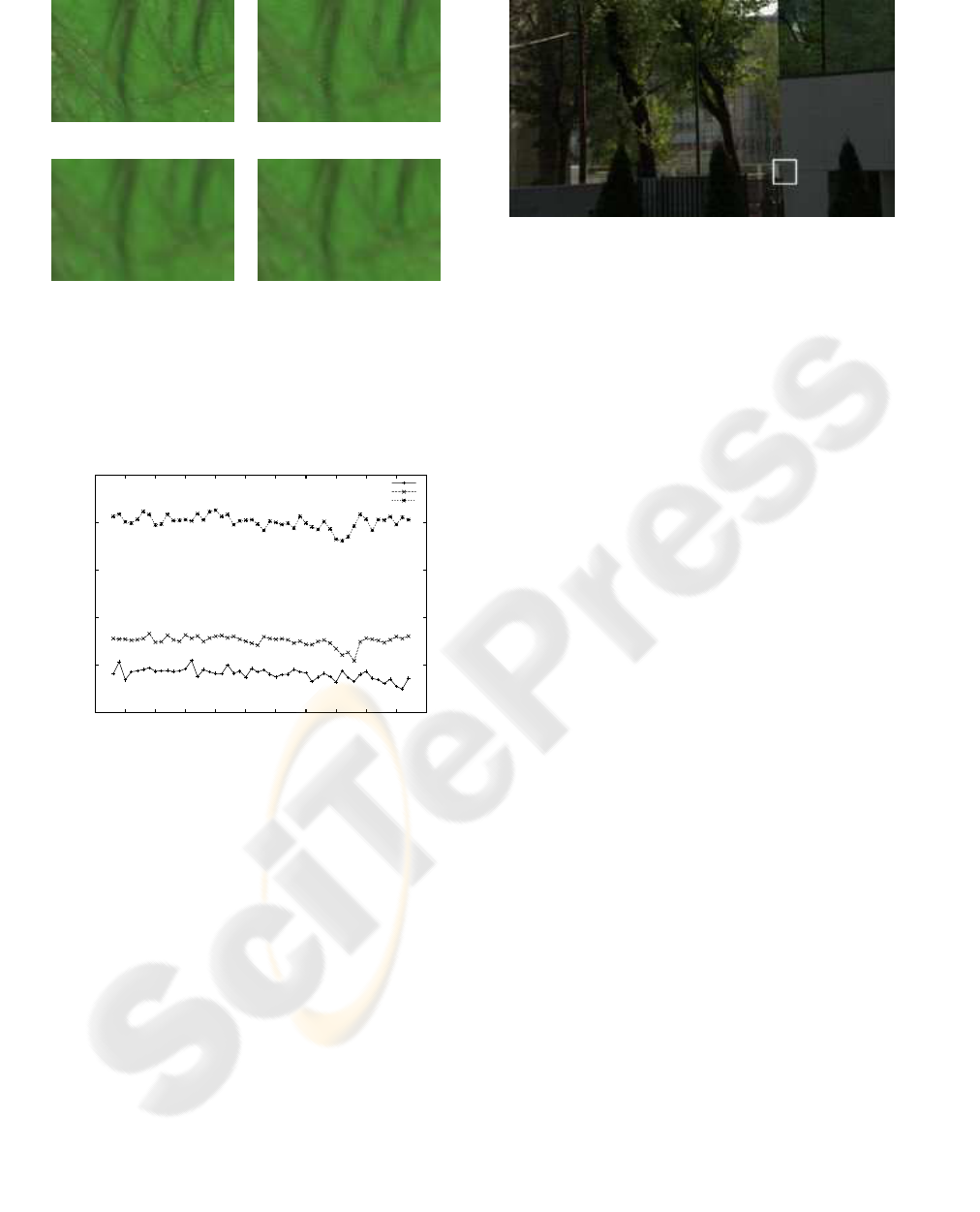
Figure 2: Reduced scale colour image from original DPX

digital cine frame from studio sequence ‘face’. Relatively

soft focus is used with a moving subject. Box indicates

where detail is shown in Figure 3. Note that this and all

following images are uncorrected log colour space.

It was observed that VQ-based enhancement

method was better than conventional method (e.g

bspline) since the latter introduces more blurriness to

the images. As an illustration, Figure 4 compares the

degree of the blurriness (expressed as blur index) of

several images from ‘outdoor’ sequence which have

been enhanced by three different methods (our pro-

posed VQ-based, bilinear, and b-spline). Note that

higher value of the blur indexon an image implies that

the image contains more blurring artifacts. It shows

that the blurriness indices of the bspline and bilinear

enhanced images are generally higher than those of

VQ-based. Figures 6 and 7 show the relative blurri-

ness of the expanded images compared to the original.

4 CONCLUSION

This paper presented a novel approach to image en-

hancement using a technique which would avoid the

known shortcomings of fractal enhancement. We

learnt the statistical properties of the co-occurrence

of low and high frequency image content and used

these probability distributions to predict image con-

Table 1: Peak-signal-to-noise ratio and weighted-peak-

signal-to-noise ratio image quality metrics for the image

expansions shewn in Figure 3. (1) Our algorithm, (2) Bi-

linear Interpolation, (3)B-Spline interpolation. Note that all

calculations are done on the 10 bit logarithmic representa-

tion used in DPX which compresses the upper part of the

dynamic range and tends to give lower PSNR values than

will be familiar from for 8 bit linear representations.

(1) (2). (3)

PSNR 16.8 dB 8.4dB 6.4 dB

WPSNR 22.9 dB 14.4dB 12.4 dB

(a) Original (b) Our algorithm

Figure 3: A region with high frequency detail from origi-

nal DPX video frame from the ’face’ sequence (a) and the

corresponding region generated by expansion of the half-

resolution video frame by our algorithm (b), as well as by

B-Spline interpolation (c) and Bilinear interpolation (d).

0.1

0.2

0.3

0.4

0.5

20 25 30 35 40 45 50 55 60 65 70 75

Blur index

Frame number

VQ-based

Bilinear

BSpline

Figure 4: Frame-by-frame blurriness comparison between

sequence of images (from ‘outdoor’ sequence) expanded

with VQ-based, bilinear, and b-spline methods.

tent during image expansion. Our algorithm out per-

forms conventional approaches based on both objec-

tive and subjective metrics, with PSNR and WPSNR

scores almost double that of the best conventional ap-

proaches. We hope to continue working on our algo-

rithm which is still in its preliminary stages by

1. Learning statistical co-occurrence of neighbour-

ing codebook blocks in images

2. Mediating the addition of high frequency pre-

dicted detail with the energy of the underlying re-

gion in the image to prevent prediction of detail in

the absence of high frequency information in the

original image.

Figure 5: Image taken outside in bright light, with sharp

focus containing more high frequency detail. Box shows

area used in Figure 6.

ACKNOWLEDGEMENTS

This work is supported by the European Commission

under the IP-RACINE project (IST-2-511316-IP).

REFERENCES

Barnsley, M. and Hurd, L. (1993). Fractal image compres-

sion. AK Peters.

Chaddha, N., Vishwanath, M., and Chou, P. (1995). Hier-

archical vector quantization of perceptually weighted

block transforms. Proceedings of the Conference on

Data Compression.

Girod, B. (1993). What’s wrong with mean-squared error?

In Watson, A. B., editor, Digital Images and Human

Vision, pages 207–220.

Gunawan, I. P. and Ghanbari, M. (2005). Image quality as-

sessment based on harmonics gain/loss information.

In Proceedings of ICIP’05 (IEEE International Con-

ference on Image Processing), volume 1, pages 429–

432, Genoa, Italia.

Levine, J., Mason, T., and Brown, D. (1992). lex & yacc.

O’Reilly & Associates, Inc. Sebastopol, CA, USA.

Linde, Y., Buzo, A., and Gray, R. (1980). An Algorithm

for Vector Quantizer Design. IEEE Transactions on

Communications, 28(1):84–95.

Pratt, W. K. (1978). Digital Image Processing. John Wiley

and Sons.

Voloshynovskiy, S., Herrigel, A., Baumg¨artner, N., and

Pun, T. (1999). A stochastic approach to content

adaptive digital image watermarking. In International

Workshop on Information Hiding, volume LNCS 1768

of Lecture Notes in Computer Science, pages 212–

236, Dresden, Germany. Springer Verlag.

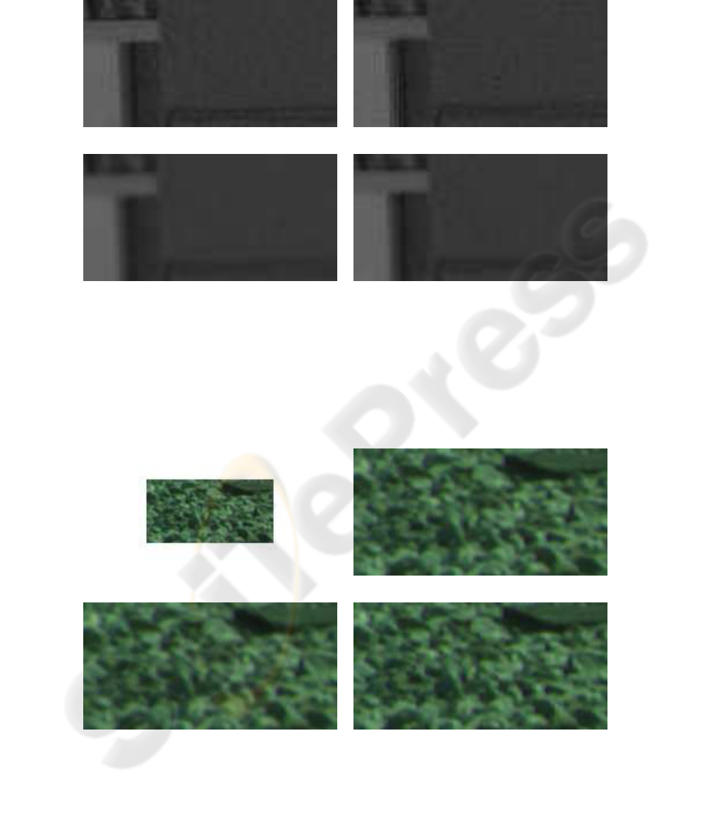
(a) Original (b) Our algorithm

Figure 6: Samples taken from the frame shown in Figure 5. The algorithm convincingly synthesises speckle on the concrete

wall but leaves the white wall in the background speckle free.

(a) Original (b) Our algorithm

Figure 7: Samples from ‘train’ sequence. The original patch (a) is taken from 2K resolution image. The patches from the

expanded images (b,c, and d) are of 4K resolution.