
AUTOMATED IMAGE ANALYSIS OF NOISY MICROARRAYS
Sharon Greenblum, Max Krucoff
Department of Biomedical Engineering, Northwestern University, Evanston, IL, USA
Jacob Furst, Daniela Raicu
School of Computer Science, Telecommunications, and Information Systems, DePaul University, Chicago, IL, USA
Keywords: DNA Microarray, image analysis, noise, segmentation, gridding, quantification, addressing, indexing.
Abstract: A recent extension of DNA microarray technology has been its use in DNA fingerprinting. Our research
involved developing an algorithm that automatically analyzes microarray images by extracting useful
information while ignoring the large amounts of noise. Our data set consisted of slides generated from DNA
strands of 24 different cultures of anthrax from isolated locations (all the same strain that differ only in
origin-specific neutral mutations). The data set was provided by Argonne National Laboratories in Illinois.
Here we present a fully automated method that classifies these isolates at least as well as the published
AMIA (Automated Microarray Image Analysis) Toolbox for MATLAB with virtually no required user
interaction or external information, greatly increasing efficiency of the image analysis.
1 INTRODUCTION
In the field of genetic analysis, DNA microarrays
have become a go-to method for studying gene
expression in an organism by measuring the ratios of
multi-channel hybridization. A recent extension of
this technology, however, is its use in DNA
fingerprinting, i.e. generating a unique pattern of
probe hybridization for an unknown DNA sequence
to compare with known DNA sequences and identify
its origin. This less-explored avenue of genetic
analysis has led to new challenges in the area of
microarray image processing, for which few
techniques have been developed.
Of the existing programs (for example, the
AMIA Toolbox for MATLAB (White, 2005)), none
are fully automated. A non-automated program may
require a sizeable amount of user input regarding
spot size, seeded region growing thresholds, array
size, control point size and location, and starting
points for grid creation. The necessity of manually
entering this information requires more background
knowledge of the slide than may be available,
influences the image processing depending on the
user running the program, and significantly slows
down the overall time required to analyze a slide.
In light of these inefficiencies and short-
comings, we present a new, fully-automated image
processing method for grayscale intensity
microarray images. In addition, we accommodate
slides with extremely low signal to noise ratios
(SNRs). Our data set consisted of slides generated
from DNA strands of 24 different cultures of anthrax
from isolated locations (all the same strain). Each
isolate contained 9 slides, each of which had four
10x10 spot arrays. In total, we analyzed 864 10x10
spot arrays on 216 separate slide images. The data
set was provided by Argonne National Laboratories
in Illinois.
2 BACKGROUND
Many microarray image processing techniques exist
that attempt to extract useful information from
images while ignoring background noise. Most
techniques divide the process into three steps:
gridding (addressing each spot), segmentation
(separating spot pixels from background pixels), and
quantification (putting spot intensity data into
numerical form for comparison).
371
Greenblum S., Krucoff M., Furst J. and Raicu D. (2007).
AUTOMATED IMAGE ANALYSIS OF NOISY MICROARRAYS.
In Proceedings of the Second International Conference on Computer Vision Theory and Applications - IFP/IA, pages 371-375
Copyright
c
SciTePress

2.1 Gridding
Because it is often easiest to analyze each 10x10
array separately, ‘super’ or ‘global’ gridding is
needed. This is the process of separating each array
into its own image. Once this is achieved, the dots
themselves can be gridded within the supergridded
array. This provides an index (or address) for each
dot (or lack thereof).
There are a number of challenges associated with
both supergridding and gridding. For example,
individual dots may be translated from a regular
array pattern due to bent or otherwise off-center
dipping pins used to create the dots. Furthermore,
some dots in a microarray image may have very
weak (or absent) intensities and may be hard to
detect. Finally, noise in the image due to elements of
the image capturing techniques (e.g. washing
techniques, dust, scratches, etc.) may interfere with
gridding algorithms.
In an attempt to tackle these challenges, various
gridding methods have been employed including
manual gridding, horizontal and vertical profiling
(Blekas, 2005), a Bayesian approach to deforming a
regular grid (Lipori, 2005; Ho, 2006), and a Markov
random field based approach (Katzer, 2003).
2.2 Segmentation
Once a spot’s location is known, separating the dot
pixels from the background pixels provides another
challenge. This process can be difficult due to
inconsistent background intensities within one image
as well as across many slides due to smudges,
overlap of extremely bright dots, and variation in
washing techniques. In addition, spot morphology is
rarely consistent and the location of a dot within a
grid box can vary considerably. Finally, weak dots
can be very hard to distinguish from a noisy
background, even visually.
Methods that have been proposed to confront
these challenges include a Hough transform to find
circles (Horsthemke, 2006), K-means clustering
(Wu, 2003) of pixels within a grid box, fixed or
adaptive circle segmentation (Yang, 2001), adaptive
ellipse methods (Rueda, 2005), adaptive shape
methods (using watershed or seeded region growing)
(Yang, 2001; Angulo, 2003), histogram
segmentation (Yang, 2001), and Gauss-Laguerre
wavelets to create an enhanced image that can be
used as a mask (Pallavaram, 2004).
2.3 Quantification
The ultimate goal of image processing is to obtain
values representative of spot intensities so that the
degree of DNA hybridization can be analyzed and
compared.
Proposed methods of addressing this challenge
include simply averaging all foreground pixel
intensities, averaging foreground pixels and
subtracting or dividing by a local or global
background intensity, fitting of a parametric model
to pixel intensities with the help of M-estimators
(Brändle, 2003) and integrating individual pixel
intensities to obtain a spot intensity reading (Bemis).
3 METHODS
When attempting to analyze real (non-ideal)
microarray images, large amounts of noise can
confound automatic algorithms. Therefore, it is
necessary to first eliminate this noise before
proceeding with further analysis. Generally
speaking, the noise inherent in these images, while
differing from image to image, has certain specific
properties that enable us to differentiate it from the
signal. Many steps in our procedure check for these
properties and use them to filter out the noise.
3.1 Addressing/Indexing
3.1.1 Supergridding
Orientation spots were used to separate the full slide
into smaller and more predictable grids. Orientation
spots are intended to be the brightest spots on the
array and are used to make sure that a slide is not
upside-down or in an incorrect orientation during
image capture (Figure 1).
Figure 1: An original slide image as visualized in
MATLAB. Only the orientation spots can be seen because
of their relative brightness.
From here we use horizontal and vertical
profiling to create a ‘supergrid’ that can be used to
crop the image (Figure 2).
VISAPP 2007 - International Conference on Computer Vision Theory and Applications
372
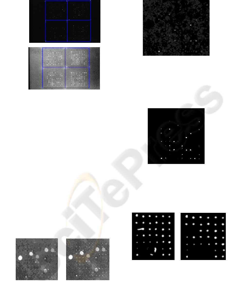
A
B
Figure 2: A) Supergrid drawn over original image. B)
Supergrid shown over enhanced image. Now we can see
the spots of interest and the four sections.
At this point, the image is cropped and each
section is analyzed separately.
3.1.2 Gridding
After the original image is cropped into its four
sections, our program grids each of the new images
separately. Our process applies a sequence of filters
to each image to ensure that any information used in
the profiling is actual data. Then we apply a set of
quality control loops that complete grids when data
is missing and eliminate rows and columns when
there is still noise included even after the filtering.
In the gridding process, we are more concerned with
eliminating false data than ignoring weak data
because this ensures that we will get a more accurate
grid. In segmentation, we look at the original,
unfiltered image, so weak data will be included.
Our process begins by applying a median filter
that helps eliminate salt and pepper noise (Figure 3).
Next we apply a disc filter similar to that applied
during supergridding (Figure 4).
A
B
Figure 3: A) Enhanced view of original crop. Notice the
salt and pepper noise. B) Same crop after median filter has
been applied. There is much less randomness to the pixel
values, and more structure has been introduced.
Figure 4: Disc filter applied to the image shown in figure
3B. Notice that the large splotches have been eliminated,
as well as any uneven illumination.
From here, we convert the image to black and
white using a thresholding technique, and the edges
of each image are cropped to remove any remnants
of the orientation spots still in the image (which are
now treated as noise—Figure 5).
Figure 5: Image with cropping at the edges. Notice the
deletions of potentially misleading data.
Since there may still be noise left in the image,
we apply our novel filters next: a ‘pixel filter’ and an
‘oblong filter’ that remove, respectively, stray pixels
and oblong shapes from the black and white image
(Figure 6).
A B
Figure 6: An example of the effectiveness of the oblong
filter at removing non-circular data. A) Black and white.
B) After oblong filter.
Now we can apply horizontal and vertical
profiles to generate a preliminary grid of the data
(Figure 7).
AUTOMATED IMAGE ANALYSIS OF NOISY MICROARRAYS
373
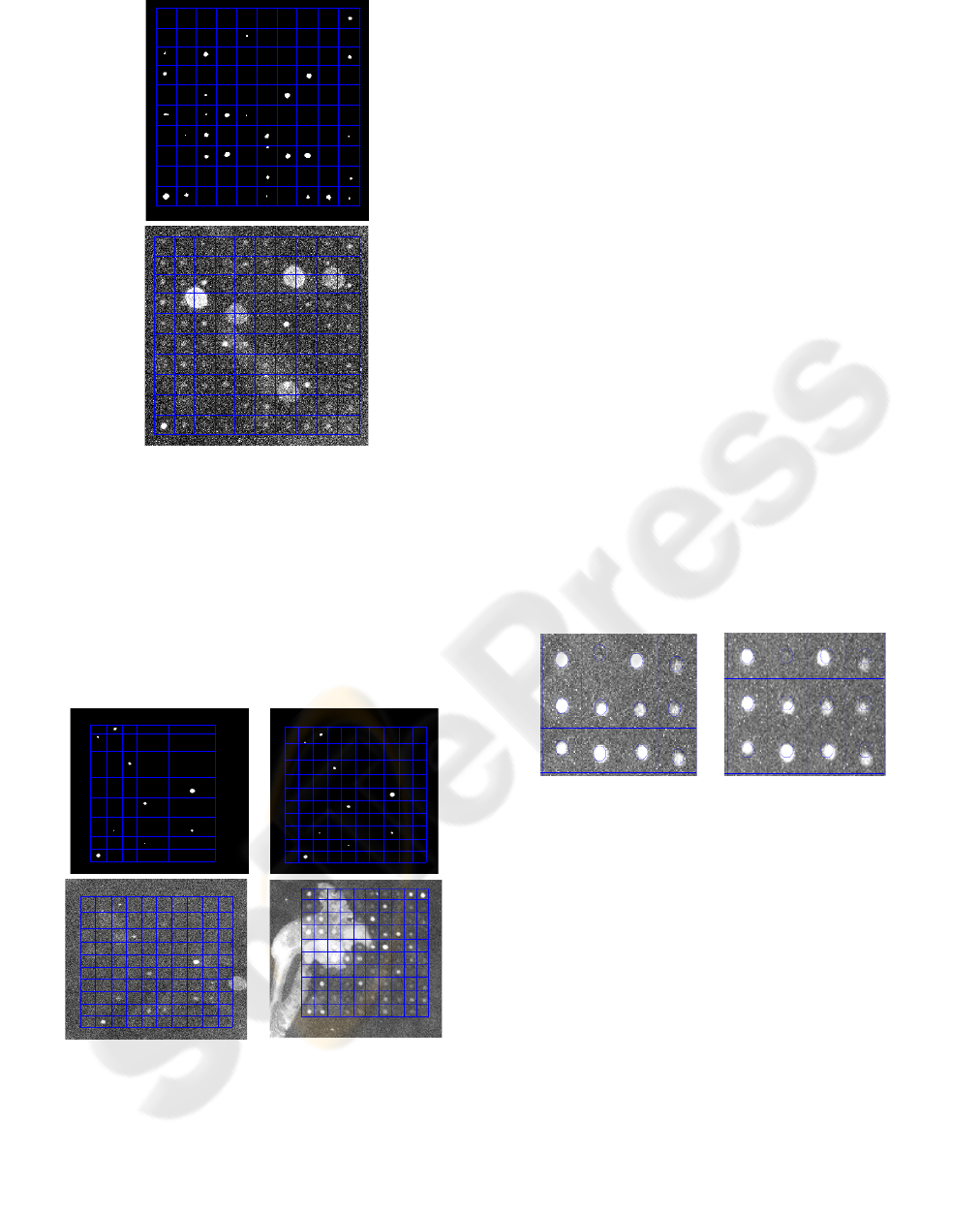
A
B
Figure 7: A) Grid shown over black and white image. B)
Grid shown over original enhanced image from Figure 3.
Notice how much noise it ignores.
Sometimes, especially when whole rows and/or
columns are absent in the original image, our grid at
this point is not satisfactory. From here, the image
runs through our novel control loops that check for
grid columns and rows that are too large and too
small, as well as grids that have too many or too
little rows and columns.
A B
C D
Figure 8: A) An example of a preliminary grid of a crop
without much useful information. B) Same slide after it
has run through our control loops. C) The final grid
shown over an enhanced view of the original crop. D)
Example of gridding results over noisy data.
The control loops then fill in missing information or
delete extraneous information based on expected
sizes of rows and columns within a certain range. If
there is enough information in the slide, the control
loops should not have to be used. However, in the
cases in which whole rows or columns are missing,
our automated program will fill them in. (Figure 8).
3.2 Spatial Segmentation
Once the image has been correctly addressed, we
would expect the spots to be approximately in the
center of each grid box. Therefore, one approach to
spatial segmentation is to use a “centered circle”
scheme. In this technique, a circle of known
diameter is drawn in the center of each grid box. All
the pixels inside the circle are considered ‘spot
pixels,’ and all the other pixels in the box are
considered ‘background pixels’ (Figure 9). We use
the original, unfiltered image for data collection.
Another approach to spatial segmentation is to
use a ‘wandering circle’ method. In this procedure,
our program takes a circle of expected spot diameter
and moves it throughout a specified area within each
grid box, searching for the maximum average
intensity. It uses this location as the spot location
(Figure 9). Again, we use the original, unfiltered
image for actual data collection.
A B
Figure 9: A) A close up view of the centered circle
approach and B) the wandering circle approach.
4 RESULTS
We compared our results to that of MATLAB’s
AMIA (Automated Microarray Image Analysis)
toolbox. The classification results were generated
using a Support Vector Machine and 9-fold cross-
validation of the data.
The centered circles approach worked the best;
the gridding correction step added a small boost to
the accuracy (total number of correct classifications
divided by the total number of replicates). The
results are shown below:
VISAPP 2007 - International Conference on Computer Vision Theory and Applications
374

Percent of Isolates Classified Correctly
Centered Circles alone: 56.28%
Grid Corrections: 56.68 %
AMIA: 55.35%
The generally low percentages may be due largely to
the poor quality of the images and the very close
similarities between the strands, not necessarily the
image processing techniques. It also may have to do
with the applied statistical methods.
Possible improvements to these results are
discussed in the future work section below.
5 CONCLUSIONS AND FUTURE
WORK
Because we found a method with at least equal
accuracy and greater automation than the AMIA
toolbox, we consider our work an improvement on
DNA microarray image processing for grayscale
intensity, noise-filled image classification. The only
user input required for our program to run all the
way through is for the user to locate the folder in the
computer that contains the images. It was surprising
to see that the wandering circle method did not
improve upon the centered circle method. One
reason for this inconsistency might be that noise has
too great an effect on circle location.
We will also investigate different statistical
approaches – the literature has shown techniques
that generate almost 90% accuracy on the AMIA
data, and we feel that more advanced statistical
analyses will generate even better results on data
generated by our algorithms.
REFERENCES
White, A., Daly, D., Willse, A., Protic M., and Chandler,
D., 2005. “Automated microarray image analysis
toolbox for MATLAB.” Bioinformatics 21:3578-3579.
Blekas, K., Galatsanos, N., Likas, A., Lagaris, I., 2005.
“Mixture model analysis of DNA microarray images.”
IEEE Trans. Med. Imaging 24(7): 901-909.
Lipori, G., 2005. “Efficient gridding of real microarray
images,” Proceedings of the Workshop on Biosignal
Processing and Classification of the International
Conference on Informatics in Control, Automation and
Robotics.
Ho, J., Hwang, W., Horn-Shing Lu, H., Lee, D., 2006.
“Gridding Spot Centers of Smoothly Distorted
Microarray Images” IEEE Transactions on Image
Processing.
Katzer, M., Kummert, F., Sagerer, G., 2003. “A Markov
random field model of microarray gridding,”
Symposium on Applied Computing, pp. 72-77.
Horsthemke, B., Furst, J., 2006. "DNA Microarray Spot
Detection Using Hough Transforms", CTI Research
Symposium.
Wu S., Yan, H., 2003. “Microarray image processing
based on clustering and morphological analysis,”
Proceedings of the First Asia-Pacific Bioinformatics
Conference on Bioinformatics, Vol. 19, pp. 111-118.
Yang, Y., Buckley, M., Speed, T., 2005. "Analysis of
cDNA microarray images," Briefings in
Bioinformatics, Vol. 2, pp. 341-349.
Rueda, L., Qin, L., 2005. “A New Method for DNA
Microarray Image Segmentation” International
Conference on Image Analysis and Recognition, pp
886-893.
Angulo, J., Serra, J., 2003. “Automatic analysis of DNA
microarray images using mathematical morphology,”
Bioinformatics 19(5): 553-562.
Pallavaram, Carli, M., Berger, J., Neri, A., Mitra, S.,
2004. "Spot identification in microarray images using
Gauss-Laguerre wavelets", Proc. IEEE Workshop on
Genomic Signal Processing and Statistics.
Brändle, N., Bischof, H., and Lapp, H., 2003. “Robust
DNA microarray image analysis,” Machine Vision
Applications.
Bemis, R., “DNA Microarray Image Processing Case
Study,” MATLAB Central.
<http://www.mathworks.com/matlabcentral/fileexchan
ge/loadFile.do?objectId=2573& objectType=FILE>
AUTOMATED IMAGE ANALYSIS OF NOISY MICROARRAYS
375
