
SIMULTANEOUS ROBUST FITTING OF MULTIPLE CURVES
Jean-Philippe Tarel
ESE, Laboratoire Central des Ponts et Chauss
´
ees, 58 Bd Lefebvre, 75015 Paris, France
Pierre Charbonnier
ERA 27 LCPC, Laboratoire des Ponts et Chauss
´
ees, 11 rue Jean Mentelin, B.P. 9, 67035 Strasbourg, France
Sio-Song Ieng
ERA 17 LCPC, Laboratoire des Ponts et Chauss
´
ees, 23 avenue de l’amiral Chauvin, B.P. 69, 49136 Les Ponts de C
´
e, France
Keywords:
Image Analysis, Statistical Approach, Robust Fitting, Multiple Fitting, Image Grouping and Segmentation.
Abstract:
In this paper, we address the problem of robustly recovering several instances of a curve model from a single
noisy data set with outliers. Using M-estimators revisited in a Lagrangian formalism, we derive an algorithm
that we call SMRF, which extends the classical Iterative Reweighted Least Squares algorithm (IRLS). Com-
pared to the IRLS, it features an extra probability ratio, which is classical in clustering algorithms, in the
expression of the weights. Potential numerical issues are tackled by banning zero probabilities in the com-
putation of the weights and by introducing a Gaussian prior on curves coefficients. Applications to camera
calibration and lane-markings tracking show the effectiveness of the SMRF algorithm, which outperforms
classical Gaussian mixture model algorithms in the presence of outliers.
1 INTRODUCTION
In this paper, we propose a method for robustly re-
covering several instances of a curve model from a
single noisy data set with severe perturbations (out-
liers). It is based on an extension of the work re-
ported in (Tarel et al., 2002), in which M-estimators
are revisited in an Lagrangian formalism which leads
to a new derivation and convergence proof of the well-
known Iterative Reweighted Least Squares (IRLS) al-
gorithm. Following the same approach based on the
Lagrangian framework, we derive, in a natural way,
a deterministic, alternate minimization algorithm, for
Simultaneous Multiple Robust Fitting (SMRF) which
extends the IRLS algorithm. Compared to the IRLS,
the SMRF features an extra probability ratio, which
is classical in clustering algorithms, in the expression
of the weights. Potential numerical issues are tack-
led by banning zero probabilities in the computation
of the weights and by introducing a Gaussian prior
on the curves coefficients. Such a prior is, moreover,
well-suited to sequential image processing and pro-
vides control on the curves. Applications to camera
calibration and lane-markings tracking illustrate the
effectiveness of the SMRF algorithm. In particular, it
outperforms classical Gaussian mixture model algo-
rithms in the presence of outliers.
The paper is organized as follows. In Sec. 2, we
present the robust multiple curves estimation problem
and introduce our algorithmic strategy. The resulting
algorithm is given in Sec. 3. Technical details on its
derivation and convergence proof are given in the Ap-
pendix. In Sec. 4, connections are made with other
approaches in the domain. Finally, we apply the al-
gorithm to road tracking and to camera calibration, in
Sec. 5.
2 MULTIPLE ROBUST
MAXIMUM LIKELIHOOD
ESTIMATION (MLE)
In this section, we model the problem of simultane-
ously fitting m curves in a robust way. Each individual
curve is explicitly described by a vector parameter
˜
A
j
,
1 ≤ j ≤ m. The observations, y, are given by a linear
generative model:
y = X(x)
t
˜
A
j
+ b (1)
where (x,y) are the image coordinates of a data point,
˜
A
j
= ( ˜a
ij
)
0≤i≤d
is the vector of curve parameters and
175
Tarel J., Charbonnier P. and Ieng S. (2007).
SIMULTANEOUS ROBUST FITTING OF MULTIPLE CURVES.
In Proceedings of the Second International Conference on Computer Vision Theory and Applications - IFP/IA, pages 175-182
Copyright
c
SciTePress

X(x) = ( f
i
(x))
0≤i≤d
is the vector of basis functions at
the image coordinate x, which will be denoted as X for
the sake of simplicity. These vectors are of size d+ 1.
Example of basis functions will be given in Sec. 5.2.
Note that we consider the fixed design case, i.e. in (1),
x is assumed non-random. In that case, it is shown
that certain M-estimators attain the maximum possi-
ble breakdown point of approximately 50% (Mizera
and M
¨
uller, 1999). In all that follows, the measure-
ment noise b is assumed independent and identically
distributed (iid) and centered. In order to render the
estimates robust to non-Gaussian noise (outliers), we
formulate the noise distribution as:
p
s
(b) ∝
1
s
e
−
1
2
φ((
b
s
)
2
)
(2)
where ∝ denotes the equality up to a factor, and s
is the scale of the pdf. As stated in (Huber, 1981),
the role of φ is to saturate the error in case of a large
noise |b| = |X
t
˜
A
j
− y|, and thus to lower the impor-
tance of outliers. The scale parameter, s, controls
the distance from which noisy measurements have a
good chance of being considered as outliers. As in the
half-quadratic approach (Geman and Reynolds, 1992;
Charbonnier et al., 1997; Tarel et al., 2002), φ(t) must
fulfill the following hypotheses:
• H0: defined and continuous on [0,+∞[ as well as
its first and second derivatives,
• H1: φ
′
(t) > 0 (thus φ is increasing),
• H2: φ
′′
(t) < 0 (thus φ is concave).
Note that these assumptions are very different from
those used in (Huber, 1981), where the convergence
proof required that the potential function ρ(b) =
φ(b
2
) be convex. In the present case, the concav-
ity and monotonicity requirements imply that φ
′
(t) is
bounded, but φ(b
2
) is not necessarily convex w.r.t. b.
Our goal is to simultaneously estimate the m curve
parameter vectors A
j=1,··· ,m
from the whole set of n
data points (x
i
,y
i
), i = 1,··· ,n. The probability of a
measurement point (x
i
,y
i
), given the m curves is the
sum of the probabilities over each curve:
p
i
((x
i
,y
i
)|A
j=1,··· ,m
) ∝
1
s
j=m
∑
j=1
e
−
1
2
φ((
X
t
i
A
j
−y
i
s
)
2
)
.
Concatening all curve parameters into a single vector
A = (A
j
), j = 1,··· , m of size m(d + 1), we can write
the probability of the whole set of points as the prod-
uct of the individual probabilities:
p((x
i
,y
i
)
i=1,···,n
|A) ∝
1
s
n
i=n
∏
i=1
j=m
∑
j=1
e
−
1
2
φ((
X
t
i
A
j
−y
i
s
)
2
)
(3)
Maximizing the likelihood p((x
i
,y
i
)
i=1,···,n
|A) is
equivalent to minimizing the negative of its logarithm:
e
MLE
(A) =
i=n
∑
i=1
−ln(
j=m
∑
j=1
e
−
1
2
φ((
X
t
i
A
j
−y
i
s
)
2
)
) + nln(s)
(4)
Using the same trick as the one described in (Tarel
et al., 2002) for robust fitting of a single curve, we
introduce the auxiliary variables w
ij
= (
X
t
i
A
j
−y
i
s
)
2
, as
explained in the Appendix. We then rewrite the value
e
MLE
(A) as the value achieved at the unique saddle
point of the following Lagrange function:
L
R
=
i=n
∑
i=1
j=m
∑
j=1
1
2
λ
ij
(w
ij
− (
X
t
i
A
j
− y
i
s
)
2
)
+
i=n
∑
i=1
ln(
j=m
∑
j=1
e
−
1
2
φ(w
ij
)
) − nln(s) (5)
Then, the algorithm obtained by alternated minimiza-
tions of the dual function w.r.t. λ
ij
and A is globally
convergent, towards a local minimum of e
MLE
(A), as
shown in the Appendix.
3 SIMULTANEOUS MULTIPLE
ROBUST FITTING
ALGORITHM
As detailed in the Appendix, minimizing (5) leads to
alternate between the three sets of equations:
w
ij
= (
X
t
i
A
j
− y
i
s
)
2
,1 ≤ i ≤ n,1 ≤ j ≤ m, (6)
λ
ij
=
e
−
1
2
φ(w
ij
)
∑
k=m
k=1
e
−
1
2
φ(w
ik
)
φ
′
(w
ij
),1 ≤ i ≤ n,1 ≤ j ≤ m,
(7)
(
i=n
∑
i=1
λ
ij
X
i
X
t
i
)A
j
=
i=n
∑
i=1
λ
ij
y
i
X
i
,1 ≤ j ≤ m (8)
In practice, some care must be taken, to avoid nu-
merical problems and singularities. First, it is impor-
tant that the denominator in (7) be numerically non-
zero, which might occur for a data point located far
from all curves. Zero probabilities are banned by
adding a small value ε (equal to the machine preci-
sion) to the exponential in the probability p
i
of a mea-
surement point. As a consequence, when a point with
index i is far from all curves, φ
′
(w
ij
) is weighted by a
constant factor, 1/m , in (7).
Second, the linear system in (8) can be singular.
To avoid this, it is necessary to enforce a Gaussian
prior on the whole curves parameters with bias A
pr

and covariance matrix C
pr
. Note that the reason for
introducing such a prior is not purely technical: it is
indeed a very simple and useful way of taking into
account application-specific a priori knowledge, as
shown in Sec. 5.3 and 5.4. A default prior can be
used. In practice, we found very useful the following
default prior: the bias is zero, i.e A
pr
= 0, and the in-
verse covariance matrix is block diagonal where each
diagonal block equals:
C
pr
−1
= r
1
−1
X(x)X(x)
t
dx (9)
assuming that [−1, 1] is the range where x varies. The
regularization term (A−A
pr
)C
pr
−1
(A− A
pr
) is added
to (4) and (5). Therefore, the parameter r allows us to
balance between the data fidelity term and the prior.
The advantage of the default prior described above is
that it is a model of the perturbations due to the image
sampling.
Finally, the Simultaneous Multiple Robust Fitting
algorithm (SMRF) is:
1. Initialize the number of curves m, the vector A
0
=
(A
0
j
), 1 ≤ j ≤ m, which gathers all curves param-
eters and set the iteration index to k = 1.
2. For all indexes i, 1 ≤ i ≤ n, and j, 1 ≤ j ≤ m,
compute the auxiliary variables w
k
ij
= (
X
t
i
A
k−1
j
−y
i
s
)
2
and the weights λ
k
ij
=
ε+e
−
1
2
φ(w
k
ij
)
mε+
∑
j=m
j=1
e
−
1
2
φ(w
k
ij
)
φ
′
(w
k
ij
).
3. Solve the linear system:
h
D+C
pr
−1
i
A
k
=
∑
i=n
i=1
λ
k
i1
y
i
X
i
.
.
.
∑
i=n
i=1
λ
k
im
y
i
X
i
+C
pr
−1
A
pr
.
4. If kA
k
−A
k−1
k > ε
′
, increment k, and go to 2, else
the solution is A = A
k
.
In the above algorithm, D is the block-diagonal
matrix whose m diagonal blocks are the matrices
∑
i=n
i=1
λ
k
ij
X
i
X
t
i
of size (d+1)×(d+1), with 1 ≤ j ≤ m.
The prior covariance matrix C
pr
is of size m(d +
1) × m(d + 1). The prior bias A
pr
is a vector of size
m(d + 1), as well as A and A
k
. The complexity is
O(nm) for the step 2, and O(m
2
(d + 1)
2
) for the step
3 of the algorithm.
4 CONNECTIONS WITH OTHER
APPROACHES
The proposed algorithm has important connections
with previous works in the field of regression and
clustering and we would like to highlight a few of
them.
In the single curve case, m = 1, the SMRF algo-
rithm is reduced to the so-called Iterative Reweighted
Least Squares extensively used in M-estimators (Hu-
ber, 1981) and half-quadratic theory (Charbonnier
et al., 1997; Geman and Reynolds, 1992). The SMRF
and IRLS algorithms share very similar structures and
it is important to notice that the main difference is
within the Lagrange multipliers λ
ij
, see (7). Com-
pared to the IRLS, the λ
ij
are just weighted by an ex-
tra probability ratio, which is classical in clustering
algorithms.
To make the connection with clustering clearer, let
us substitute Y = A
j
+ b to the generative model (1),
where Y and A
j
are vectors of same size and respec-
tively denote a data points and a cluster centroid. The
derivation described in Sec. 3 is still valid and the
obtained algorithm turns to be a clustering algorithm
with m clusters, each cluster being represented by a
vector, its centroid. The probability distribution of a
cluster around its centroid is directly specified by the
function φ. The obtained algorithm is thus able of
modeling the Y
i
’s by a mixture of pdfs which are not
necessarily Gaussian. The mixture problem is usually
solved by the well-known Expectation-Minimization
(EM) approach (Dempster et al., 1977). In the non-
Gaussian case, the minimization (M) step implements
robust estimation, which is an iterative process in it-
self. Hence, the resulting EM algorithm involves two
nested loops, while the proposed algorithm features
only one. An alternative to the EM approach is the
Generalized EM (GEM) approach which consists in
performing an approximate M-step: typically, only
one iteration rather than the full minimization. The re-
sulting algorithm in the robust case is identical to the
one we derived in the Lagrangian framework (apart
from the regularization of the singular cases). In our
formalism however, no approximation is made in the
derivation of the algorithm, in contrast with the GEM
approach.
We also found that the SMRF algorithm is very
close to an earlier work in the context of cluster-
ing (Cambell, 1984). However, to our knowledge, the
latter was just introduced as an extra ad-hoc weight-
ing over M-estimators without statistical interpreta-
tion and, moreover, singular configurations were not
dealt with.
The SMRF algorithm is subject to the initializa-
tion problem since it only converges towards a lo-
cal minimum. To tackle this problem, the Graduated
Non Convexity approach (GNC) (Blake and Zisser-
man, 1987) is used to improve the chances of converg-
ing towards the global minimum. Details are given
in Sec. 5.4. The SMRF can be also used as a fitting
process within the RANSAC (Hartley and Zisserman,
2004) approach to improve the convergence towards
the global minimum.
5 EXPERIMENTAL RESULTS
The proposed approach being based on a linear gen-
erative model, many applications could potentially be
addressed using the SMRF algorithm. In this paper,
we focus on two specific applications, namely simul-
taneous lane-markings tracking and camera calibra-
tion from a regular lattice of lines with geometric dis-
tortions.
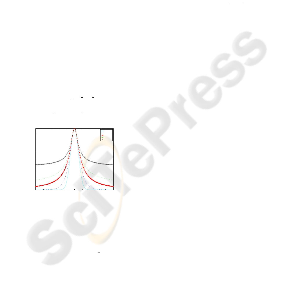
5.1 Noise Model
Among the suitable functions for robust estimation,
we use a simple parametric family of probability dis-
tribution functions, that was introduced in (Tarel et al.,
2002) under the name of smooth exponential family
(SEF), S
α,s
:
S
α,s
(b) ∝
1
s
e
−
1
2
φ
α
((
b
s
)
2
)
(10)
where, with t = (
b
s
)
2
, φ
α
(t) =
1
α
((1+t)
α
− 1).
−10 −8 −6 −4 −2 0 2 4 6 8 10
0
0.1
0.2
0.3
0.4
0.5
0.6
0.7
0.8
0.9
1
S
α,s
distribution
α = 1
α = 0.5
α = 0.1
α = −0.1
α = −0.5
Figure 1: Noise models in the SEF S
α,s
. Notice how the
tails become heavier as α decreases.
These laws are shown in Figure 1 for different val-
ues of α. The smaller the value of α, the higher the
probability of observing large, not to say very large,
errors (outliers). This parameter allows a continuous
transition between well-known statistical laws such as
Gauss (α = 1), smooth Laplace (α =
1
2
) and T-Student
(α → 0). This can be exploited to get better conver-
gence of the SMRF algorithm by using the GNC ap-
proach, i.e. by progressively decreasing α towards 0.
5.2 Road Shape Model
The road shape features (x, y) are given by the lane-
marking centers extracted using the local feature ex-
tractor described in (Ieng et al., 2004). An exam-
ple of extraction is shown in Figure 6(b). In prac-
tice, we model road lane markings by polynomials
y =
∑
d
i=0
a
i
x
i
. Moreover, in the flat world approxi-
mation, the image of a polynomial on the road un-
der perspective projection is a hyperbolic polynomial
with equation y = c
0
x+ c
1
+
∑
d
i=2
c
i
(x−x
h
)
i
, where c
i
is
linearly related to a
i
. Therefore, the hyperbolic poly-
nomial model is well suited to the case of road scene
analysis. To avoid numerical problems, a whitening
of the data is performed by scaling the image in a
[−1,1] × [−1, 1] box for polynomial curves and in a
[0,1] × [−1,1] box for hyperbolic polynomials, prior
to the fitting.
5.3 Geometric Priors
As noticed in Sec. 3, the use of a Gaussian prior al-
lows introducing useful application-specific knowl-
edge. For example, using (9) for the diagonal blocks
of the inverse prior covariance matrix, we take into
account perturbations due to image sampling.
Tuning the diagonal elements of C
pr
provides con-
trol on the curve degree. For polynomials, the diago-
nal components of the covariance matrix correspond
to monomials of different degrees. The components
of degree higher than one are thus set to smaller val-
ues than those of degree zero and one.
Geometric smooth constraints between curves can
be enforced by using also non-zero off-diagonal
blocks, in particular it is a way of maintaining paral-
lelism between curves. As an illustration, to smoothly
enforce parallelism between two lines y = a
0
+ a
1
x
and y = a
′
0
+ a
′
1
x, the prior covariance matrix is ob-
tained by rewriting (a
1
− a
′
1
)
2
in matrix notations:
a
0
a
1
a
′
0
a
′
1
t
0 0 0 0
0 1 0 −1
0 0 0 0
0 −1 0 1
a
0
a
1
a
′
0
a
′
1
The above matrix, multiplied by an overall factor can
be used as an inverse prior covariance C
pr
−1
. The
factor controls the balance between the data fidelity
term and the other priors. Other kinds of geomet-
ric smooth constraints can be handled in a similar
way, such as intersection at a given point, or symmet-
ric orientations. These geometric priors can be com-
bined by adding the associated regularization term
(A− A
pr
)C
pr
−1
(A− A
pr
) to (4).
5.4 Lane-Markings Tracking
We shall now describe the application of the SMRF
algorithm to the problem of tracking lane markings.
In addition to the previous section, another inter-
esting feature of using a Gaussian prior is that the
SMRF is naturally suitable for being included in a
Kalman filtering. However, this raises the question
of the definition of the posterior covariance matrix
of the estimate. Under the Gaussian noise assump-
tion, the estimate of the posterior covariance matrix
is well-known for each curve: C
j
= s
2
∑
i=n
i=1
X
i
X
t
i
−1
.
Unfortunately, in the context of robust estimation, the
estimation of C
j
for each curve A
j
is a difficult issue
and only approximate matrices are available. In (Ieng
et al., 2004), several approximates were compared.
The underlying assumption for defining all these ap-
proximates is that the noise is independent. How-
ever, we found out that in practice, the noise is cor-
related from one image line to another. Therefore,
all these approximates can be improved by introduc-
ing an had-hoc correction factor which accounts for
data noise correlations in the inverse covariance ma-
trix. We found experimentally that the following fac-
tor is appropriate, for each curve j:
1−
∑
i=n−1
i=1
p
λ
ij
w
ij
λ
i+1, j
w
i+1, j
∑
i=n
i=1
λ
ij
w
ij
The approximate posterior covariance matrix for the
whole set of curve parameters, A, is simply built as
a block-diagonal matrix made of the individual pos-
terior covariance matrices for each curve, C
j
. This
temporal prior can be easily combined with geometric
priors to allow tracking of parallel curves for instance.
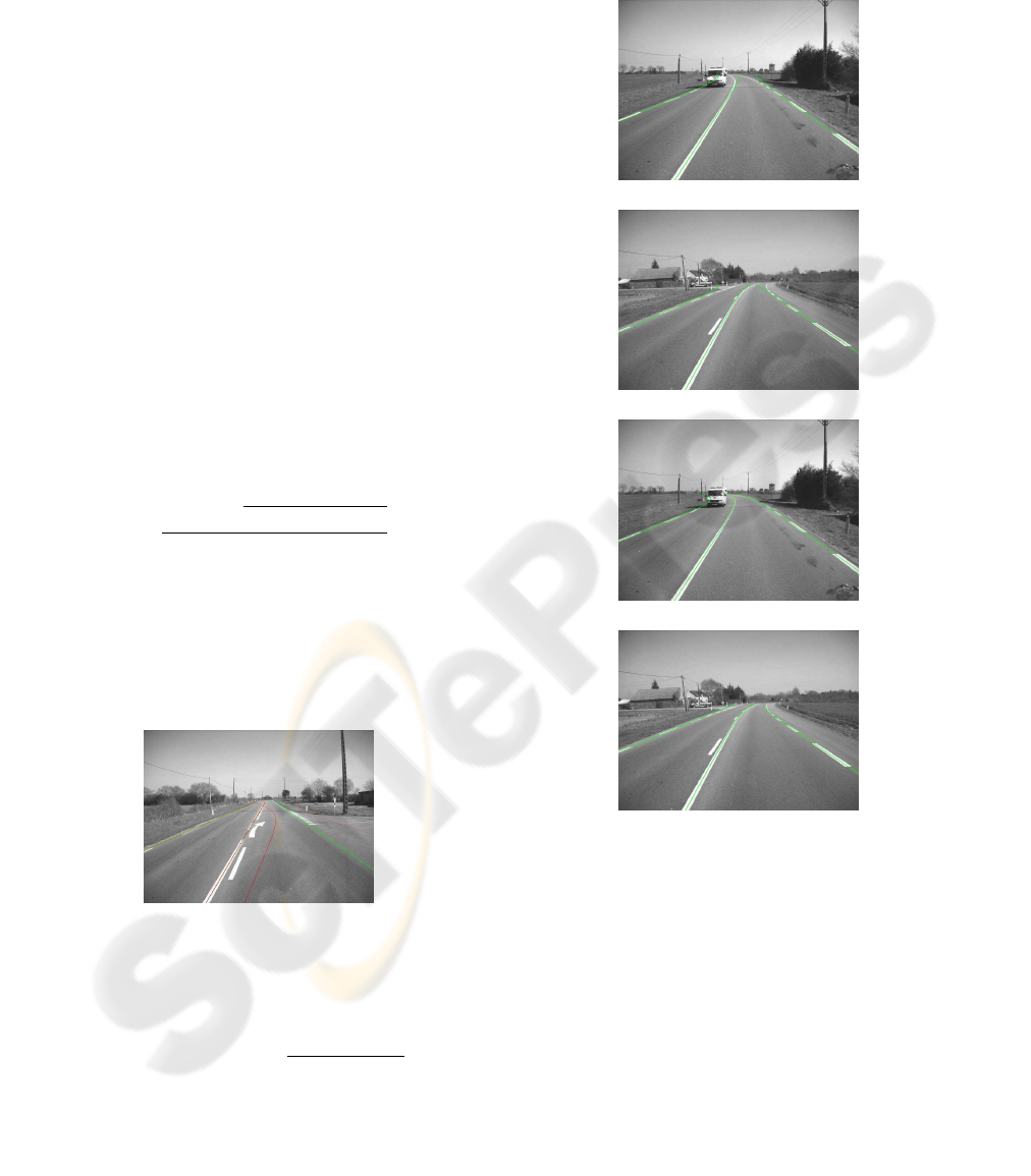
Figure 2: Detected lane-markings (in green) and uncer-
tainty about curve position (in red).
Figure 2 shows the three curves simultaneously
fitted on the lane-marking centers (in green) and the
associated uncertainty curves of the horizontal posi-
tion of each fitted curve (±
q
X(x)
t
C
−1
j
X(x), in red).
Notice that the uncertainty on the right sparse lane-
marking is higher than for the continuous one on
the center. Moreover, the higher the distance to the
camera, the higher the uncertainty, since the curve
gets closer to possible outliers. In all these exper-
iments, and following, the parameters used for the
noise model are α = 0.1 and s = 4.
(a)
(b)
(c)
(d)
Figure 3: Two images extracted from a sequence of 240 im-
ages processed with, on (a)(b), separate Kalman filters and,
on (c)(d), simultaneous Kalman filter. The three detected
lane-markings of degree two are in green.
For the tracking itself, we experimented both sep-
arate Kalman filters on individual curves, and a si-
multaneous Kalman filter. The former can be seen
as a particular case of the latter, in which the inverse
prior covariance matrix C
pr
is block-diagonal so the
linear system of size m(d+ 1) in the SMRF algorithm
can be decomposed as m linear independent systems
of size d + 1. Figure 3 compares the results obtained
with separate and simultaneous Kalman filters. No-
tice how the parallelism between curves is better pre-
served within the simultaneous Kalman filter, thanks
to an adequate choice of the off-diagonal blocks of
C
pr
.
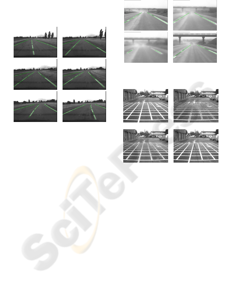
Figure 4: Six of a 150-image sequence, featuring lane
changes. Green lines show the three fitted lane-markings
centers.
Figure 4 illustrates the ability of the SMRF-based
Kalman filter to fit and track several curves in an
image sequence. In that case, three lane-markings
are simultaneously fitted and correctly tracked, even
though the vehicle performs several lane changes
during the 150-image sequence. Notice that, while
Kalman filtering can incorporate a dynamic model of
the vehicle, we only used a static model in these ex-
periments, since only the images were available. We
observed that it is better to initialize the SMRF algo-
rithm with the parameters resulting from the fitting
on the previous image, rather than with the filtered
parameters: filtering indeed introduces a delay in the
case of fast displacements or variations of the tracked
curves.
Moreover, we obtained interesting results on dif-
ficult road sequences. For instance, Figure 5 shows
a short sequence of poor quality images, due to rain.
The left lane-marking is mostly hidden on two con-
secutive images. Thanks to the simultaneous Kalman
filter, the SMRF algorithm is able to interpolate cor-
rectly the hidden lane-marking.
5.5 Camera Calibration
We now present another application of the SMRF al-
gorithm, in the context of camera calibration. The
Figure 5: Fitting in adverse conditions: in this excerpt,
the left lane-marking is mostly hidden on two successive
images.
(a) (b)
(c) (d)
Figure 6: (a) Original image of the calibration grid. (b) Ex-
tracted lane-marking centers (outliers are due to puddles).
(c) 10 initial lines for the fitting on the vertical markings. (d)
Fitted lines on the vertical markings under Gaussian noise
assumption.
goal is to estimate accurately the position and orien-
tation of the camera with respect to the road and its
intrinsic parameters. A calibration setup made of two
sets of perpendicular lines painted on the road is thus
observed by a camera mounted on a vehicle, as shown
in Figure 6(a). The SMRF algorithm can be used to
provide accurate data to the calibration algorithm by
estimating the grid intersections. Even though the
markings are clearly visible in the image, some of
them are quite short, and there are outliers due to the
presence of water puddles. Figure 6(b) shows the ex-
tracted lane-marking centers. When a Gaussian mix-
ture model is used, the obtained fit is severely trou-
bled by the outliers, as displayed in Figure 6(d), even
though the curves are initialized very close to the ex-
pected solution, see Figure 6(c).
On the contrary, with the same extracted lane-

(a) (b)
(c) (d)
Figure 7: (a) 12 initial lines for the fitting on the vertical
markings. (b) The fitting yields 11 different lines. (c) 12
second degree polynomials fitted on the horizontal mark-
ings. (d) Results of the horizontal and vertical fitting super-
imposed.
marking centers, the SMRF algorithm, with noise
model parameters α = 0.1 and s = 4, leads to nice
results, as shown in Figure 7(b) for the vertical lines,
and in Figure 7(c) for the horizontal curves. 11 dif-
ferent lines were obtained for the vertical markings,
and 12 different second degree polynomials were ob-
tained for the horizontal markings. Figure 7(d) shows
the two sets of curves superimposed.
We also use these calibration images to investigate
the issue of initialization. We typically take a num-
ber of curve prototypes higher than the real number
of curves in the image, see e.g. Figure 7(a). We ob-
served that the extra prototypes may be either fitted on
outliers groups or identical to another fitted prototype
(e.g. in Figure 7(b), two resulting curves are identi-
cal). Detecting identical curves is easy, for instance
by performing a Bayesian recognition test on every
pair (A
j
,A
k
), i.e. comparing (A
j
− A
k
)
t
C
−1
j
(A
j
− A
k
)
to a small threshold, where C
j
is the posterior covari-
ance matrix of the curve A
j
. To detect prototypes fit-
ted to only a few points such as outliers, we exploit
the uncertainty measure provided by the posterior co-
variance matrix and simply threshold −log(det(C
j
)).
Finally, notice that the SMRF algorithm does not re-
quire to be initialized very close to the expected solu-
tion, as illustrated by Figure 7(a)(b).
6 CONCLUSION
In the continuing quest for achieving robustness in
detection and tracking curves in images, this pa-
per makes two contributions. The first one is the
derivation, in a MLE approach and using Kuhn and
Tucker’s classical theorem, of the so-called SMRF al-
gorithm. This algorithm extends mixture model algo-
rithm, such as the one derived using EM, to robust
curve fitting. It is also an extended version of the
IRLS, in which the weights incorporate an extra prob-
ability ratio. The second contribution is the regular-
ization of the SMRF algorithm by introducing Gaus-
sian priors on curve parameters and the handling of
potential numerical issues by banning zero probabil-
ities in the computation of weights. From our exper-
iments, banning zero probabilities seems to have im-
portant positive consequences in pushing the curves
to spread out all the data, and thus in providing im-
proved robustness to the initialization, as shown in
the context of camera calibration. The introduction
of the Gaussian prior is also beneficial in particu-
lar in the context of image sequence processing, as
illustrated with an application of simultaneous lane-
markings tracking on-board a vehicle in adverse con-
ditions. The approach being based on a linear gener-
ative model, it is quite generic and we believe that it
can be used with benefits in many other fields, such
as clustering or appearance modeling.
REFERENCES
Blake, A. and Zisserman, A. (1987). Visual Reconstruction.
MIT Press, Cambridge, MA.
Boyd, S. and Vandenberghe, L. (2004). Convex Optimiza-
tion. Cambridge University Press.
Cambell, N. A. (1984). Mixture models and atypycal val-
ues. Mathematical Geology, 16(5):465–477.
Charbonnier, P., Blanc-F
´
eraud, L., Aubert, G., and Barlaud,
M. (1997). Deterministic edge-preserving regulariza-
tion in computed imaging. IEEE Transactions on Im-
age Processing, 6(2):298–311.
Dempster, A., Laird, N., and Rubin, D. (1977). Maxi-
mum likelihood from incomplete data via the EM al-
gorithm. Journal of the Royal Statistical Society, Se-
ries B (Methodological), 39(1):1–38.
Geman, D. and Reynolds, G. (1992). Constrained restora-
tion and the recovery of discontinuities. IEEE Trans-
actions on Pattern Analysis and Machine Intelligence,
14(3):367–383.
Hartley, R. I. and Zisserman, A. (2004). Multiple View Ge-
ometry in Computer Vision. Cambridge University
Press, ISBN: 0521540518, second edition.
Huber, P. J. (1981). Robust Statistics. John Wiley and Sons,
New York, New York.
Ieng, S.-S., Tarel, J.-P., and Charbonnier, P. (2004). Eval-
uation of robust fitting based detection. In Proceed-
ings of European Conference on Computer Vision
(ECCV’04), pages 341–352, Prague, Czech Republic.

Luenberger, D. G. (1973). Introduction to linear and non-
linear programming. Addison Wesley.
Minoux, M. (1986). Mathematical Programming: Theory
and Algorithms. Chichester: John Wiley and Sons.
Mizera, I. and M
¨
uller, C. (1999). Breakdown points and
variation exponents of robust m-estimators in linear
models. The Annals of Statistics, 27(4):1164–1177.
Tarel, J.-P., Ieng, S.-S., and Charbonnier, P. (2002). Us-
ing robust estimation algorithms for tracking explicit
curves. In European Conference on Computer Vision
(ECCV’02), volume 1, pages 492–507, Copenhagen,
Danmark.
APPENDIX
We shall first rewrite the value −e
MLE
(A) for any
given A = (A
j
), j = 1,··· ,m as the value achieved
at the minimum of a convex problem under convex
constraints. This is obtained by introducing the aux-
iliary variables w
ij
= (
X
t
i
A
j
−y
i
s
)
2
. This apparent com-
plication is in fact valuable since it allows us to in-
troduce Lagrange multipliers, and thus to decompose
the original problem in simpler problems. The value
−e
MLE
(A) can be seen as the minimum value, w.r.t.
W = (w
ij
)
1≤i≤n,1≤ j≤m
, of:
E(A,W) =
i=n
∑
i=1
ln(
j=m
∑
j=1
e
−
1
2
φ(w
ij
)
)
subject to nm constraints h
ij
(A,W) = w
ij
−
(
X
t
i
A
j
−y
i
s
)
2
≤ 0. This is proved by showing that
the bound on each w
ij
is always achieved. Indeed
E(A,W) is decreasing w.r.t. each w
ij
, since its first
derivative:
∂E
∂w
ij
= −
1
2
e
−
1
2
φ(w
ij
)
∑
k=m
k=1
e
−
1
2
φ(w
ik
)
φ
′
(w
ij
)
is always negative, due to (H1).
To prove the local convergence of the SMRF algo-
rithm in Sec. 3, we now focus on the minimization of
E(A,W) w.r.t. W only, subject to the nm constraints
h
ij
(A,W) ≤ 0, w.r.t. W, for any A. We now introduce
a classical result of convex analysis (Boyd and Van-
denberghe, 2004): the function g(Z) = log(
∑
j=m
j=1
e
z
j
)
is convex. Due to (H1) and (H2), −φ(w) is convex and
decreasing. Therefore, E(A,W) w.r.t. W is convex as
a sum of functions g composed with −φ, see (Boyd
and Vandenberghe, 2004). As a consequence, the
minimization of E(A,W) w.r.t. W is well-posed be-
cause it is a minimization of a convex function subject
to convex (linear) constraints. We are thus allowed
to apply Kuhn and Tucker’s classical theorem (Mi-
noux, 1986): if a solution exists, the minimization of
E(A,W) w.r.t. W is equivalent to searching from the
unique saddle point of the Lagrange function of the
problem:
L
R
(A,W,Λ) =
i=n
∑
i=1
ln(
j=m
∑
j=1
e
−
1
2
φ(w
ij
)
)
+
i=n
∑
i=1
m
∑
j=1
1
2
λ
ij
(w
ij
− (
X
t
i
A
j
− y
i
s
)
2
)
where Λ = (λ
ij
),1 ≤ i ≤ n, 1 ≤ j ≤ m are Kuhn and
Tucker multipliers (λ
ij
≥ 0). More formally, we have
proved for any A:
−e
MLE
(A) = min
W
max
Λ
L
R
(A,W,Λ) (11)
Notice that the Lagrange function L
R
is quadratic
w.r.t. A, unlike the original error e
MLE
. Using the sad-
dle point property, we can change the order of vari-
ables W and Λ in (11). We now introduce the dual
function
E (A, Λ) = min
W
L
R
(A,W,Λ), and rewrite the
original problem as the equivalent following problem:
min
A
e
MLE
(A) = min
A,Λ
−
E (A, Λ)
The algorithm consists in minimizing −
E (A, Λ) w.r.t.
A and Λ alternately. min
Λ
−
E (A, Λ) leads to Kuhn
and Tucker’s conditions:
λ
ij
=
e
−
1
2
φ(w
ij
)
∑
k=m
k=1
e
−
1
2
φ(w
ik
)
φ
′
(w
ij
) (12)
w
ij
= (
X
t
i
A
j
− y
i
s
)
2
(13)
and min
A
j
−
E (A, Λ) leads to:
(
i=n
∑
i=1
λ
ij
X
i
X
t
i
)A
j
=
i=n
∑
i=1
λ
ij
y
i
X
i
, 1 ≤ j ≤ m (14)
Using classical results, see e.g. (Minoux, 1986),
−
E (A, Λ) is proved to be convex w.r.t. Λ. The dual
function is clearly quadratic and convex w.r.t. A. As
a consequence, this implies that such an algorithm al-
ways strictly decreases the dual function if the current
point is not a stationary point (i.e a point where the
first derivatives are all zero) of the dual function (Lu-
enberger, 1973). The problem of stationary points is
easy to solve by checking the positiveness of the Hes-
sian matrix of
E (A, Λ). If this matrix is not positive,
we disturb the solution so that it converges to a local
minimum. This proves that the algorithm is globally
convergent, i.e, it converges toward a local minimum
of e
MLE
(A) for all initial A
0
’s which are neither a max-
imum nor a saddle point.
