HUE VARIANCE PREDICTION

An Empirical Estimate of the Variance within the Hue of an Image

Robert N. Grant, Richard D. Green and Adrian J. Clark

Dept. Computer Science, University of Canterbury, Christchurch, New Zealand

Keywords:

Hue noise, image processing, illumination invariance.

Abstract:

In the area of vision-based local environment mapping, inconsistent lighting can interfere with a robust system.

The HLS colour model can be useful when working with varying illumination as it tries to separate illumination

levels from hue. This means that using hue information can result in an image invariant to illumination. This

can be valuable when trying to determine object boundaries, object identiﬁcation and image correspondence.

The problem is that noise is greater at lower illumination levels. While removing the illumination effects on

the image, separating out hue means that the noise effects of non-optimal illumination remain. This paper

looks at how the known illumination information of pixels can be used to accurately predict and reduce noise

in the hue obtained in video from a colour digital camera.

1 INTRODUCTION

With vision-based local environment mapping consis-

tency in the environment is highly desirable. This

includes consistent lighting conditions which means

that most research is conducted under as controlled

an environment as possible. Unfortunately this is

not a luxury that can be afforded in real world ap-

plications which means that many projects can not

achieve widespread public use. The problem is that

illumination in general usage is unpredictable, caus-

ing tasks such as colour tracking for object recogni-

tion to be problematic because the intrinsic charac-

teristics of digital cameras causes the value of hue to

vary with illumination. There have been projects in

the past that have tried to track the colour of an object

as it changes with varying levels of success (Grant

and Green, 2004)(Nummiaro et al., 2002)(Vergs-Llah

et al., 2001) shown in ﬁgure 1. While these methods

can work, they often need to be reinitialised if track-

ing is lost and are computationally inefﬁcient leaving

less for the primary vision application.

This research takes the approach of an illumina-

tion invariant ﬁlter on video data, acquiring video

frames and converting them into a normalised illu-

mination format consisting of the raw colours of the

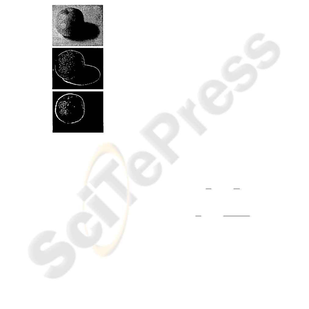
Figure 1: Frames from a dynamic colour tracker (Grant and

Green, 2004).

scene. Conversion to the HLS colour model shown in

ﬁgure 2 is the starting point to this transformation as

the hue component of this colour model is essentially

the colour of an object with the illumination inten-

sity information stripped out. White balancing is also

necessary to remove light source colouring effects on

objects.

This would be an ideal illumination invariant input

for a computer vision system as with accurate white

N. Grant R., D. Green R. and J. Clark A. (2007).

HUE VARIANCE PREDICTION - An Empirical Estimate of the Variance within the Hue of an Image.

In Proceedings of the Second International Conference on Computer Vision Theory and Applications - IFP/IA, pages 5-9

 SciTePress

correct the effects of discoloured lighting in an image

(Lam et al., 2004).

By implementing reliable white balancing and

using an invariant colour model an object’s colour

should rarely change due to illumination changes.

Unfortunately this is not the case when the intensity

of light reﬂected from an object nears the outer limits

of the camera’s visible range. Cameras are not sensi-

tive to these areas and so noise causes the colour/hue

of an object to vary dramatically.

Figure 4: Shadow segmentation using an invariant colour

model (Salvador et al., 2001).

3 EXPERIMENTATION

3.1 Method

The following experiment aims to discover the corre-

lation between the effect of noise levels on hue and

the levels of the other two components of HLS colour

(luminance and saturation). These may be useful pre-

dictors as they represent the amounts of light coming

into the camera and an indication of the accuracy of

hue. A predictable correlation between these two fac-

tors enables countering these noise effects.

Different scenes were selected for range of colour

and brightness. The camera exposure period was up

to 30 seconds at a frame rate of approximately 15fps

to collect accurate HLS colour information for each

pixel of the scene over time. Each pixel was classi-

ﬁed by means of averaging to a speciﬁc luminance

and saturation pair. Standard deviation of the hue val-

ues collected were calculated for each pixel. Hue vari-

ances are added to an array of minimum hue variance

for each luminance by saturation pair (256x256).

3.2 Results

Figure 5(a) shows the data extracted from this exper-

iment. It can be seen that at low and high luminance

and low saturation values with results indicating that

the amount of noise in hue can spike signiﬁcantly.

There are also some scattered hue noise peaks in the

data as can be seen in the graph. These can be at-

tributed to other effects caused by the method of data

collection. With a near stationary camera, tiny move-

ments can cause large changes in pixel colour near the

edges of objects. Because of this the lowest variance

is always selected when duplicate luminance and sat-

uration pairs arise, this helps reduce these effects.

These results suggest that it is possible to correctly

predict the noise of a pixel without any temporal in-

formation. Luminance and saturation may therefore

be accurate predictors of the hue variance for any

given pixel.

3.3 Curve Fitting

From the data found in ﬁgure 5(a) we can see that,

with the correct formula, hue variation can be pre-

dicted. The problem is ﬁnding this ﬁtting a mathemat-

ical curve to this data. By analysing a cross section of

the data along one axis at a time, it was found that

both axes closely ﬁt an inverse squared curve which

when multiplied together produced a close ﬁt to the

data. In the case of the luminance direction the sym-

metry means the term L is inverted half way.

When L < 128:

H = (

+ β)× (

+ δ) (1)

Else:

H = (

+ β) × (

(255 − L)

+ δ) (2)

To match the data from the previous experiment,

the coefﬁcients found to be a close ﬁt were: α = 2913,

β = 1.18, γ = 1974, δ = 0.6301. This produces the

predicted graph in ﬁgure 5(b). These coefﬁcients

would be different for different cameras but the equa-

tion should still be the same. Each camera would need

to be calibrated for a speciﬁc noise curve.

3.4 Application

Figure 6 shows the different stages of this being ap-

plied to a frame of video beginning with ﬁgure 6(a).

HUE VARIANCE PREDICTION - An Empirical Estimate of the Variance within the Hue of an Image

Figure 6(b) shows the image with only the hue com-

ponent remaining, this was done by converting to

HLS then setting luminance to 128 and saturation to

255 and then converting it back into the RGB colour

space. Figure 6(c) is formed by applying the equa-

tions 1 and 2 to the luminance and saturation from

the original image. This is then combined with the

hue image to form the image shown in ﬁgure 6(d).

(a)

(b)

Figure 5: Hue standard deviation vs. Saturation and Lumi-

nance (a) Experimental results (b) Predicted curve.

This image gives an indication as to how reliable the

colour data is and gives us an ideal entry into noise

reduction, edge detection, frame correlation or object

segmentation algorithms.

(a)

(b)

(c)

(d)

Figure 6: (a) Original image (b) Hue image (c) Predicted

hue noise image (d) Hue image with darkened noisy areas.

VISAPP 2007 - International Conference on Computer Vision Theory and Applications

4 CONCLUSIONS

This research is working towards creating an illumi-

nation invariance ﬁlter for colour camera input. This

can be used to better identify or correlate objects re-

gardless of changes in lighting conditions or viewing

angle. While white balancing and illumination invari-

ant colour models are on the way to achieving this,

they come across large amounts of noise when trying

to identify colours that have intensities outside of the

sensitive range of the camera. This research has reme-

died this by showing that an equation can be used to

predict how reliable colour values are across an im-

age. In this way correlation between a persistent rep-

resentation and the camera input can be made more

reliably.

5 FUTURE WORK

Now with colour error being accurately predicted in

video, further applications of this research can take

into account this noise and operate more robustly for

it. The current two directions of research following

on from this are image enhancement and frame cor-

relation. Using the overlaps of variance for neigh-

bouring pixels, a pixels colour and variance estimates

are narrowed to become more accurate. This means

slight variations in colour across an object due to cam-

era noise are minimised resulting in a cleaner image

for viewing or vision systems. Frame correlation be-

comes simpler as the computed variance of the pixel

will generally encompass the detected colour of same

physical point in following frames.

REFERENCES

Fintzel, K., Bendahan, R., Vestri, C., Bougnoux, S., Ya-

mamoto, S., and Kakinami, T. (2003). 3d vision sys-

tem for vehicles. In Intelligent Vehicles Symposium,

2003. Proceedings. IEEE, pages 174–179.

Grant, R. N. and Green, R. D. (2004). Tracking colour

movement through colour space for real time human

motion capture to drive an avatar. In Proceedings of

Image and Vision Computing New Zealand.

Lam, H.-K., Au, O. C., and Wong, C.-W. (2004). Automatic

white balancing using standard deviation of rgb com-

ponents. In International Symposium on Circuits and

Systems, volume 3, pages 921–924.

Nummiaro, K., Koller-Meier, E., and Gool, L. J. V. (2002).

Object tracking with an adaptive color-based particle

ﬁlter. In Annual Symposium of the German Associa-

tion for Pattern Recognition, page 353 ff.

Salvador, E., Cavallaro, A., and Ebrahimi, T. (2001).

Shadow identiﬁcation and classiﬁcation using invari-

ant color models. In IEEE International Conference

on Acoustics, Speech, and Signal Processing, vol-

ume 3, pages 1545–1548.

Takeno, J. and Hachiyama, S. (1992). A collision-avoidance

robot mounting ldm stereo vision. In Proceedings of

the IEEE International Conference on Robotics and

Automation, 1992., volume 2, pages 1740–1752.

Tsuji, T., Hattori, H., Watanabe, M., and Nagaoka, N.

(2002). Development of night-vision system. In IEEE

Transactions on Intelligent Transportation Systems,

volume 3, pages 203–209.

Vergs-Llah, J., Aranda, J., and Sanfeliu, A. (2001). Object

tracking system using colour histograms. In Proceed-

ings of the 9th Spanish Symposium on Pattern Recog-

nition and Image Analysis, pages 225–230.

Wang, J. M., Chung, Y. C., Chang, C. L., and Chen, S. W.

(2004). Shadow detection and removal for trafﬁc im-

ages. In IEEE International Conference on Network-

ing, Sensing and Control, volume 1, pages 649–654.

Yao, J. and Zhang, Z. (2004). Systematic static shadow

detection. In International Conference on IPattern

Recognition, volume 2, pages 76–79.

HUE VARIANCE PREDICTION - An Empirical Estimate of the Variance within the Hue of an Image