
PRACTICAL SINGLE VIEW METROLOGY FOR CUBOIDS
Nick Pears, Paul Wright and Chris Bailey
Department of Computer Science, University of York, UK
Keywords:
Single View Metrology. 3D measurement. Feature detection. Planar homographys. Projective invariants.
Abstract:
Generally it is impossible to determine the size of an object from a single image due to the depth-scale ambi-
guity problem. However, with knowledge of the geometry of the scene and the existence of known reference
dimensions in the image, it is possible to infer the real world dimensions of objects with only a single im-
age. In this paper, we investigate different methods of automatically determining the dimensions of cuboids
(rectangular boxes) from a single image, using a novel reference target. In particular, two approaches will be
considered: the first will use the cross-ratio projective invariant and the other will use the planar homography.
The accuracy of the measurements will be evaluated in the presence of noise in the feature points. The effects
of lens distortions on the accuracy of the measurements will be investigated. Automatic feature detection
techniques will also be considered.
1 INTRODUCTION
Historically, many package delivery companies have
priced the delivery of packages mainly by weight.
However, increasingly, tariffs are related to the size
of the package being delivered, as the cost of ship-
ping the package is more closely related to how much
space it takes up in the delivery chain. If there were
a simple and fast method to establish and log into the
company’s IT system the size of a package, then great
benefits in terms of the whole system’s efficiency can
be achieved. We note that, already, package han-
dling staff often carry around mobile computer de-
vices called PDAs (personal digital assistants) to log
packages into the IT system and such devices are now
easily and readily equipped with cameras. This paper
aims to prove the principle that it is possible to mea-
sure the dimensions of a package from a single image
(for example, taken by a camera-equipped handheld
PDA), given a simple, portable reference target.
Measurement using images is termed visual
metrology and this has been studied extensively in
the computer vision literature (Criminisi et al., 1999),
(Criminisi, 2001), (Chen et al., 2006). In this paper,
we aim to automatically measure the dimensions of
cuboids (rectangular boxes) from a single image, us-
ing a simple, novel reference object attached to one
corner of the cuboid. The term automatically is used
here to mean that the only piece of information that
should be given to the system is the image of the scene
containing a box.
Several problems need to be addressed to build
such a measurement system. These include the re-
moval of distortions caused by the lens of the camera,
feature detection and identification, and dimension
measurement. Each problem will need to be solved
to produce a system that can provide accurate, auto-
matic measurements.
This paper will look at two particular methods to
compute the dimensions of a box: the cross-ratio in-
variant and the planar homography. For this type of
measuring system to be of practical use, as is the case
with all measuring systems, the results it returns have
to be accurate and reliable. It is therefore important to
assess the reliability of both techniques being investi-
gated.
The remainder of the paper is structured as fol-
lows. In section 2, we describe the two measurement
techniques, which we aim to compare. In section 3,
we describe the implementation of our measurement
system. In section 4, we present results of both sim-
ulations and real measurements and a final section is
used for conclusions.
85
Pears N., Wright P. and Bailey C. (2007).
PRACTICAL SINGLE VIEW METROLOGY FOR CUBOIDS.
In Proceedings of the Second International Conference on Computer Vision Theory and Applications - IU/MTSV, pages 85-90
Copyright
c
SciTePress
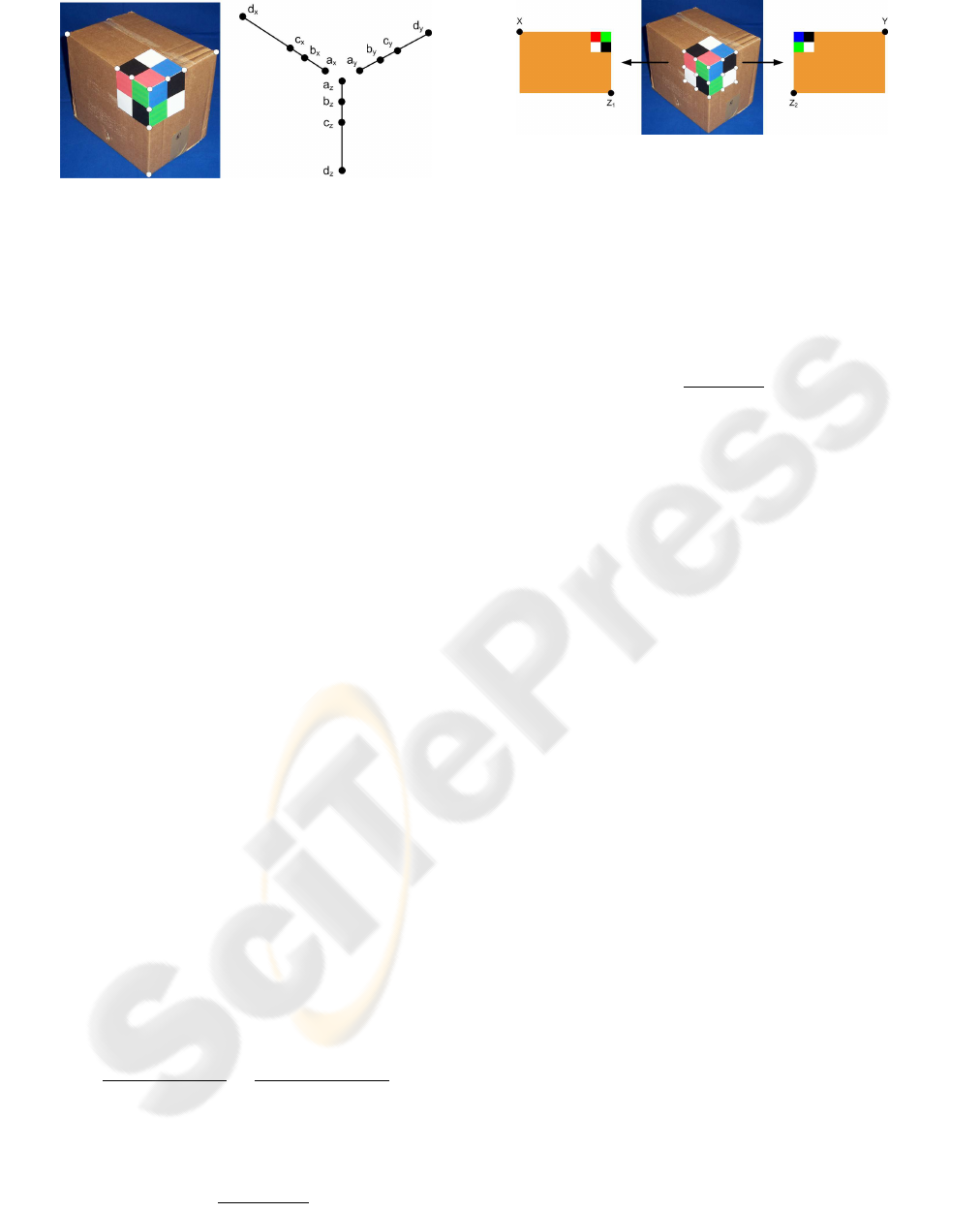
Figure 1: Cross ratio based measurement.
2 MEASUREMENT TECHNIQUES
The reference target used consists of three mutually
orthogonal, equally sized square faces, coloured with
a 2x2 chessboard pattern on each face, as shown in
fig 1. The size of the squares within the pattern are
40mm. Our target is constructed of cardboard, but
in a practical PDA-based system, we envisage that a
rugged and foldable plastic target may be used.
The colours within the reference target were care-
fully selected, so that adjacent squares in the pat-
tern have high contrast in greyscale, which allows,
for example, reliable corner detection. Target cor-
ners are identified from their normalised colour his-
tograms within a local circular neighbourhood. If all
the corners in the target are detected, this gives rise
to nine points on each target plane and three points
along each axis.
2.1 Metrology Using Invariants
Figure 1 shows an image of a box to be measured,
with the reference target in-situ. The reference points
that need to be detected in the image are shown
by white dots along three mutually orthogonal axes.
These image points are labelled (a
i
− d
i
), as shown,
where i is the one of the dimensions (x, y, z).
If we represent world coordinates as
(A
i
, B
i
,C
i
, D
i
), corresponding to image points
(a
i
, b
i
, c
i
, d
i
) along dimension i, then we can write an
equation for the invariance of the cross-ratio under
the imaging process. Using the notation d(., .) to
represent the Euclidean distance between a pair of
points, then (Hartley and Zisserman, 2000)
d(a
i
, c
i
)d(b
i
, d
i
)
d(b
i
, c
i
)d(a
i
, d
i
)
=
d(A
i
,C
i
)d(B
i
, D
i
)
d(B
i
,C
i
)d(A
i
, D
i
)
(1)
If one of the four squares on a target face has di-
mension α, then
I
i
=
2α(M
i
− α)
αM
i
(2)
Figure 2: Homography based measurement.
where I
i
is the invariant computed from image mea-
surements along the i dimension and M
i
is the un-
known measurement of the box in the i dimension,
expressed in the same units as α (typically we use
millimetres). Rearranging this equation, we have
M
i
=
α
(1− 0.5I
i
)
(3)
2.2 Metrology Using Homographys
The second method of calculating the box dimensions
uses the planar homography approach, and in par-
ticular, the normalised Direct Linear Transformation
method is used (Hartley and Zisserman, 2000).
In contrast to the cross ratio invariant, which uses
three edges of the box, the planar homography instead
uses planes of the box. Since each plane is bounded
by two axes of the box, each plane can provide a max-
imum of two dimensions of the box. Therefore a min-
imum of two planes need to be visible in order to cal-
culate all three dimensions of the box from a single
image as shown in Figure 2.
Since two planes are required for all three dimen-
sions of the box to be recovered, this means that two
homographies will need to be calculated, due to each
plane of the box undergoing a different projective
transformation during the imaging process.
The relative world position of the reference tar-
get corners are known, and through feature detection,
their corresponding image positions can be extracted
from the image. This means that the target can pro-
vide nine point correspondences per plane - more than
the minimum of four (no three collinear) required to
calculate a planar homography.
Once the homographies have been calculated, the
real world position of any point on either plane of the
box can be determined. Since the external corners of
the box lie on these planes, their real world position
can be determined through the homography. The cor-
ner relating to the height exists on both planes, so ei-
ther plane can be used to calculate this dimension, or
alternatively, an average taken.
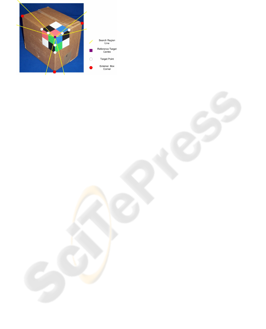
Figure 3: Feature points required for the cross ratio.
3 IMPLEMENTATION
Our system is implemented in MATLAB with the fol-
lowing the main stages:
(i) Image acquistion: A Kodak LS743 digital cam-
era was used to collect images, using the wide angle
lens setting. After capture, images are reduced from
2304 x 1728 down to 800 x 600 to reduce image pro-
cessing time.
(ii) Camera Distortion Correction: The MATLAB
Camera Calibration Toolkit (Bouguet, 2005) was used
to correct the radial distortions in the input images.
Our calibration results showed that radial distortion
has the greatest effect towards the corners of the im-
age where there are displacements of up to 50 pixels.
The effects of tangential distortions are much smaller
with only a maximum displacement of 2 pixels. With
the camera intrinsics calculated, any image can then
be corrected by the toolkit.
(iii) Corner Detection: The implementation of the
Harris corner detector (Harris and Stephens, 1988) by
Peter Kovesi (Kovesi, 2000) was used. Other interest
point detectors could also be used such as the SUSAN
detector (Smith and Brady, 1995).
(iv) Feature Point Recognition: Figure 3 illus-
trates the points required to calculate the cross ratios.
The first feature we try to identify is the central
point of the reference target, using the surrounding
colours. Colour modelling is an area that has been
researched extensively in computer vision (Alexan-
der, 1999). The approach used here is similar to that
used by Coughlan et al (Coughlan et al., 2005). For
each candidate corner, three points p
1
, p
2
and p
3
are
specified at fixed offsets, separated by 120 degrees,
such that each point is positioned in a region of red,
green or blue colour. If the letters R
i
, G
i
and B
i
rep-
resent the red, green and blue intensity values at point
p
i
, then the colour target is detected if the following
four inequalities are met: R
1
> R
2
+T, G
1
+T < G
2
,
G
2
> G
3
+ T, R
1
> R
3
+ T, where T is a threshold
value used to control the detection. It should be noted
that use of this technique does require the reference
target to be placed on the box in a specific way such
that the red region is always at the top. This approach
produces accurate and reliable detection of the target.
Once the centre of the reference target has been iden-
tified, the next step is to search for the surrounding
three points of the target that sit on the axes of the
box. These can be used to determine the direction of
the three axes of the box. These points are found in
a similar way to finding the centre of the reference
target, although different colour regions need to be
specified for each of the points.
Along each axis, the location of two points is now
known, so an approximate direction of each axis can
be calculated. The placement of the reference target
on the corner of the box is unlikely to be perfect due to
deformations of the box. Thus a search region along
each axis is determined in which to find the other re-
quired points. This search region narrows down the
number of corners that will have to be investigated.
The third point on the reference target can now be lo-
cated, again using the colour region method.
The external corner of the box is found by
analysing the colour in the region next to each corner
detected in the search region. It is assumed that close
to the edge of a box, the colour and texture of the box
should remain roughly the same. It is also assumed
that the box colour should be markedly different to
that of its background. The image is first converted
from RGB space to HSI space. A histogram of the
hue for a small region next to the final point detected
on the reference target is then obtained.
For each corner detected in the search region, a
histogram for the surrounding region is obtained. This
corner histogram is then compared to the histogram of
the region next to the target previously stored. If the
two histograms are different by some margin, then the
detected corner is likely to be a corner of the box.
(v) Metrology Calculations: The cross ratio
method was straightforward to implement. From the
set of image point coordinates, the distances between
them were calculated and the values put into equation
3 to obtain each dimension of the box. The planar
homography method used the normalised DLT algo-
rithm to estimate a homography matrix for each plane.
Then the image coordinates of the box corners were
converted into the real world coordinates, which was
used to compute the length of a side of a box. Both
planes can be used to obtain the height measurement
of the box, so the average of the two values obtained
from both planes is used as the height measurement.

Figure 4: Th effect of radial distortion.
4 RESULTS AND EVALUATION
4.1 Radial Distortion Correction
To what extent does radial distortion affect the mea-
surements and do the correction techniques employed
reduce these errors? To answer these questions, a
marked calibration plane was set up in front of the
camera so that it almost entirely filled the captured
image. The image was then corrected for radial dis-
tortion and both the uncorrected and corrected im-
ages were stored. The position in the image of each
30 mm graduation along both the x and y axes was
selected by eye. Each 30 mm graduation is consid-
ered to be the box corner, allowing the trend in mea-
surement error across the image to be observed. For
each graduation mark in both the uncorrected and cor-
rected image, its estimated position was calculated
and stored using both the cross ratio and planar ho-
mography methods.
The error in the measurements for both methods in
both the uncorrected and corrected images are shown
in Figure 4. Both the results in the x and y axis of the
plane were very similar, so Figure 4 only shows the
results obtained from the x axis. From this graph it is
clearly visible that radial distortion has a noticeable
effect on the accuracy of the results obtained from
both methods. For the uncorrected cases, the errors
start low, but increase rapidly to as much as 3.75%.
Note, however, that the radial distortion correction
significantly improves the accuracy of the results and,
for both the planar homography and cross ratio tech-
niques, the measurement errors stay relatively con-
stant across the entire calibration grid.
4.2 Comparison of Methods
Twenty two boxes were selected, ensuring a mixture
of small and large boxes and boxes with different as-
pect ratios. Images of each were captured from three
Figure 5: Comparison of actual and computed measure-
ments for 22 boxes in view 1.
views, the first of which (view 1) was such that the
camera was pointing directly through the diagonal of
the box. Each captured image was corrected for radial
distortion and feature points on the reference target
and the box corners were selected. The dimensions
of the box were then obtained from both the cross ra-
tio and planar homography methods. Firstly, the ac-
curacy of both methods will be compared. Figure 5
shows the difference between the real measurement
and the measurements estimated by both techniques
for just the width of the box. The central diagonal
(black) line shows the ideal situation where the vi-
sual metrology is perfect and there are no errors in
the measurements. The points with square markers
(green) show the measurements made using the cross
ratio for each of the 22 boxes. The points with tri-
angular markers (red) show the measurements made
using the planar homography technique. Linear least
squares trend lines for both sets of measurements are
shown.
Note that the measurements obtained are in gen-
eral close to the correct value, although they suffer
from both systematic and random error. In many ways
it is unreasonable to expect highly accurate answers,
since it can be difficult to position the reference target
on the box so that it lies flat on the plane. This is due
to the fact that the boxes are not perfectly cuboid and
the corners can be deformed. Interestingly, the sys-
tematic errors show a definite trend for the cross ratio
to overestimate the measurement whereas the planar
homography underestimates, although both of these
effects can be calibrated out, such that the trend lines
for both methods are coincident with the true mea-
surements.
From the graph, the repeatability of the measure-
ments made by both the cross ratio and planar ho-
mography methods can be compared. This can be
achieved by looking at the spread of points from their
trend line. The planar homography method produces
more stable estimations since the points are situated
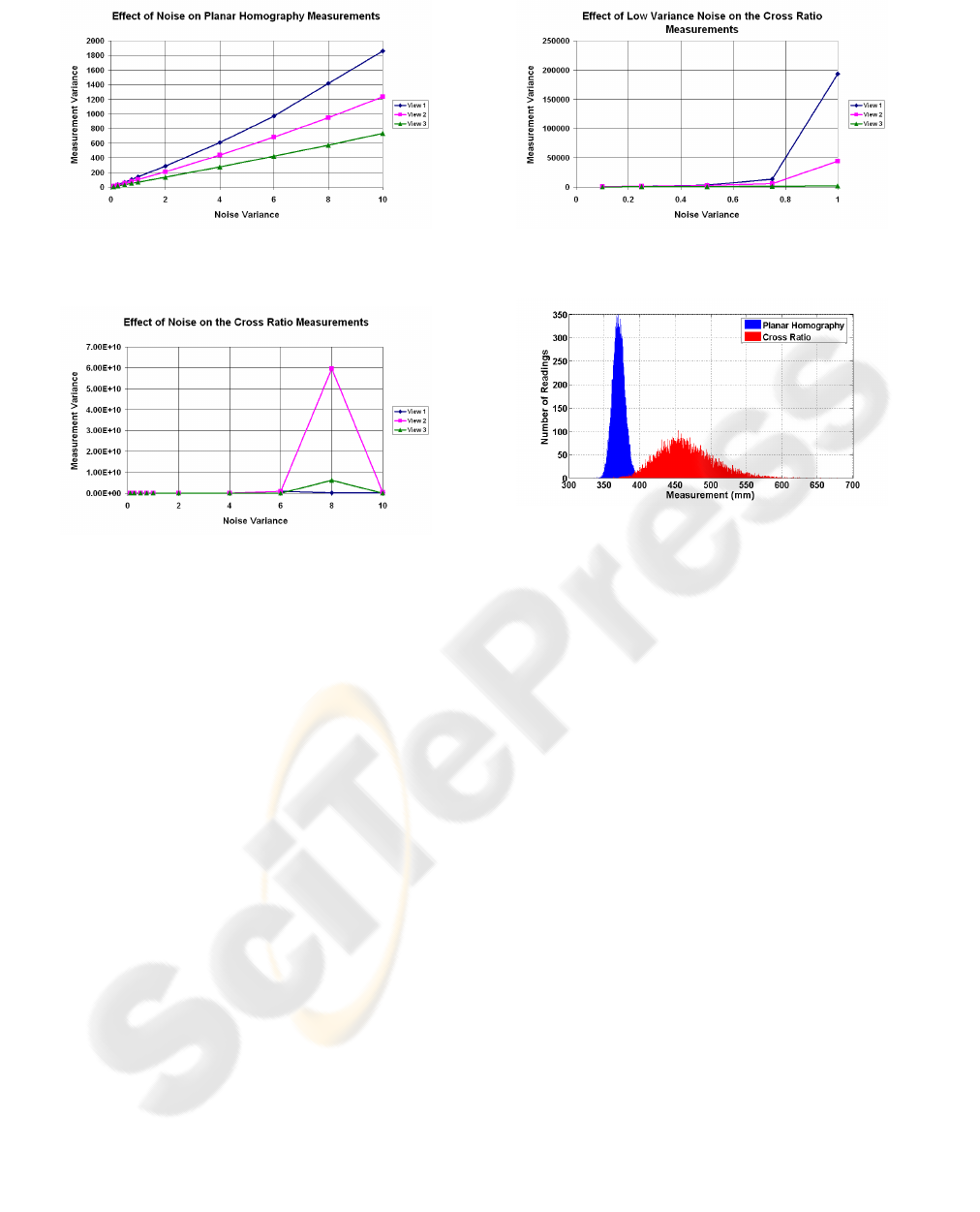
Figure 6: Effect of noise on planar homography measure-
ments.
Figure 7: Effect of noise on cross ratio measurements.
closer to its trend line. However, for the cross ratio
method, the points are often situated further from the
trend line, with their distance increasing further from
the trend line as the size of the box increases and the
relative size of the imaged reference target decreases.
4.3 Noise Sensitivity
Within the context of this work, noise will be de-
fined as movements of the detected feature points
from their expected (ideal) positions. A noise sensi-
tivity experiment was conducted as follows. For each
of the 22 undistorted test box images, the points of
the reference target and the box corners were sub-
jected to Gaussian noise with a certain variance. The
dimensions of the box were then calculated using
both the cross ratio and the planar homography tech-
niques. These measurements were stored and the fea-
ture points subjected to a new set of noise. This was
repeated 10,000 times, so 20,000 measurements were
recorded in total. This whole procedure was then re-
peated for noise variances of 0.1, 0.25, 0.5, 0.75, 1,
2, 4, 6, 8 and 10. (Note that only the width measure-
ment is used in this experiment.) For each set of mea-
surements, a series of statistics were generated such
as the average, variance and standard deviation. In
the following figures the noise variance is in (pixel
Figure 8: Effect of low variance noise on the cross ratio
measurements.
Figure 9: Histogram comparing effect of noise on the two
methods.
position)
2
and the measurement variance is in (mm)
2
.
The effects of noise on the planar homography
method will first be considered. Figure 6 shows the
variance of the width measurement as a function of
noise variance. We note that, although the planar ho-
mography is definitely susceptible to the effects of
noise, its effects are predictable. The difference in the
curves for the three views can be attributed to the fact
that going from view one (camera pointing along box
diagonal) to view 2 (camera pointing at front edge, no
top plane, width and depth have equal image size) to
view three (as view 2, but width has larger image size
than depth) favours more accurate measuring of the
width of the box.
Figure 7 shows the effects of noise on the cross ra-
tio method. Here the noise presents a much more seri-
ous problem. Not only is the variance in the measure-
ments much greater now than for the planar homog-
raphy, the relationship between the amount of noise
and measurement variance is significantly more non-
linear. This is seen clearly in Figure 8 which shows
the effects of low variance noise only.
Another way in which the data from this exper-
iment can be analysed is using a histogram to show
the spread of the results obtained from both methods.
Figure 9 shows the histogram of the results obtained
from the width measurement of a particular box. The
mean position of the two histograms is different due

to the difference in the systematic error of the under-
lying measurement made by both techniques (see Fig-
ure 5). However, this graph shows a clear difference
in the repeatability of the two methods in the presence
of noise. Whereas the planar homography histogram
is tall and narrow, the cross ratio histogram is short
and wide. This indicates that planar homography is
less sensitive to noise that the cross ratio method.
5 CONCLUSIONS
We have presented a novel reference target method for
the measurement of cuboid (box) dimensions, with a
view to producing a PDA-based system in the near
future. Using corner features on this target, we have
outlined two methods that can be used to measure box
dimensions from a single image: the cross ratio in-
variant and planar homography. Accuracies of around
5.3% show that, although our prototype is not highly
precise, it has sufficient accuracy for logging approx-
imate parcel dimensions in a parcel delivery IT sys-
tem, which can greatly improve resource planning in
the delivery chain. We conclude by answering five
important questions.
1. How accurately can box measurements be made?
For view 2, average errors of 6.7% for the
cross-ratio method and 5.3% for the homography
method were measured. This is a reasonable level
of accuracy to expect considering that it is diffi-
cult to align the reference target on the corner of a
possibly non-cuboid box. Furthermore, accuracy
may be improved by calibrating out systematic er-
rors in each method.
2. Can the required features of a box be detected reli-
ably? We have not fully answered the question of
whether completely automatic measurements can
be made. It is accepted that the feature detection
methods used in this project are basic in compari-
son to others available, which, could for example
involve SIFT features (Lowe, 2004) and pay more
attention to colour modelling (Alexander, 1999).
However, for the cross ratio method it has been
shown that it is possible to detect the required fea-
ture points automatically, although this is only re-
liable on plain boxes (no patterns or text).
3. What are the ideal conditions for measurements?
For the most accurate measuring, the three lines
required for the cross ratio or the two planes re-
quired for the planar homography should occupy
as large an area of the image as possible.
4. How are the measurements altered in the presence
of noise in the input? The measurements made by
both the cross ratio and the planar homography
methods have been investigated when the posi-
tions of the feature points are subject to noise. We
found that the cross ratio method is much more
sensitive to the effects of noise than the planar ho-
mography method.
5. Do the effects of camera distortion affect the ac-
curacy of the measurements and can the effects of
the distortions be corrected or minimised? The
problems of radial distortion have been investi-
gated and it has been shown that this form of dis-
tortion has an effect on the accuracy of the mea-
surements. Radial distortion can be corrected and
performing this operation removes significant in-
accuracy in the measurements (as much as 3% er-
ror). It is therefore imperative that radial distor-
tion is corrected before a measurement is made
from the image.
REFERENCES
Alexander, D. (1999). Advances in daylight statistical
colour modelling. In Proc. Conf. Computer Vision and
Pattern Recognition, pages 313–318.
Bouguet, J. (2005). Camera calibra-
tion toolbox for matlab 2005. url:
http://www.vision.caltech.edu/bouguetj/calib-doc/.
Chen, Z., Pears, N. E., and Liang, B. (2006). A method of
visual metrology from uncalibrated images. Pattern
Recognition Letters, 27(13):1447–1456.
Coughlan, J., Manduchi, R., Mutsuzaki, M., and Shen, H.
(2005). Rapid and robust algorithms for detecting
colour targets. In Proc. 10th Congress of the Inter-
national Colour Association.
Criminisi, A. (2001). Accurate visual metrology from single
and multiple uncalibrated images. Springer.
Criminisi, A., Reid, I., and Zisserman, A. (1999). Single
view metrology. In Proc. 7th Int. Conf. on Computer
Vision, pages 434–442.
Harris, C. J. and Stephens, M. (1988). A combined cor-
ner and edge detector. In 4th Alvey Vision Conference
Manchester, pages 147–151.
Hartley, R. I. and Zisserman, A. (2000). Multiple View Ge-
ometry in Computer Vision. Cambridge University
Press.
Kovesi, P. D. (2000). Matlab and octave functions
for computer vision and image processing. url:
http://www.csse.uwa.edu.au/ pk/research/matlabfns/.
Lowe, D. G. (2004). Distinctive image features from scale-
invariant keypoints. International Journal of Com-
puter Vision, 2(60):91–110.
Smith, S. M. and Brady, J. M. (1995). Susan-a new ap-
proach to low-level image processing. Int. Journal of
Computer Vision, 23(1):45–78.
