
AUTOMATED SEPARATION OF REFLECTIONS FROM A SINGLE
IMAGE BASED ON EDGE CLASSIFICATION
Kenji Hara, Kohei Inoue and Kiichi Urahama
Department of Visual Communication Design, Kyushu University, Fukuoka, Japan
Keywords:
Reflection separation, transparency, edge classification, pyramid structure, deterministic annealing.
Abstract:
Looking through a window, the object behind the window is often disturbed by a reflection of another object.
In the paper, we present a new method for separating reflections from a single image. Most existing techniques
require the programmer to create an image database or require the user to manually provide the position and
layer information of feature points in the input image, and thus suffer from being extremely laborious. Our
method is realized by classifying edges in the input image based on the belonging layer and formalizing the
problem of decomposing the single image into two layer images as an optimization problem easier to solve
based on this classification, and then solving this optimization with a pyramid structure and deterministic
annealing. As a result, we are able to accomplish almost fully automated separation of reflections from a
single image.
1 INTRODUCTION
One can see that the scene observed through a flat
transparent plate such as window glass normally con-
sists of a combination of two images: the reflected
image and the transmitted image. In recent years, de-
composing the superimposed image into the two im-
ages has been a topic of significant interest in the com-
puter vision community because of both its practical
importance and its theoretical difficulty.
The great difficulty of the image decomposition
problem lies in its high illposedness, since the num-
ber of unknowns (twice the number of pixels) is much
larger than the number of available constraints (the
number of pixels) (Levin et al., 2004a). Thus, much
of the image decomposition methods enforce addi-
tional constraints such as using as inputs two im-
ages taken through a polarizer at different orienta-
tions or using an image sequence taken from a video
camera (Farid and Adelson, 1999; Irani and Peleg,
1992; Sarel and Irani, 2004b; Sarel and Irani, 2004a;
Szeliski et al., 2000; Tsin et al., 2003; Schechner
et al., 2000)D
More recently, Levin et al. (Levin et al., 2004a)
developed a method for decomposing the input image
into two images from a single image. This method is
based on a prior that prefers decompositions that min-
imize a linear combination of the numbers of edges
and corners. In this work, they showed that the sin-
gle image decomposition problem can be solved even
without a priori knowledge about content or scene
contents. Also at the same period, they proposed a
user-guided semi-automatic method, which work well
even on complex images that may be difficult for the
above method to decompose (Levin et al., 2004b).
These previous works, however, require the pro-
grammer to create a database of natural images or re-
quire the user to manually provide the position and
layer information of feature points in the input image.
Hence, they suffer from the problems that the manual
data entry tasks are extremely laborious and tedious
and that the separation results may depend on the set
of images in the database.
In this paper, we present a single image decom-
position method that requires less labor, such as im-
age database construction or a considerable amount
of user interaction. In order to reduce the ambiguity
of the solution, we make the following assumptions
within Levin et al’s prior framework: (1) both of the
layers have edges, (2) the edge of a layer does not
18
Hara K., Inoue K. and Urahama K. (2007).
AUTOMATED SEPARATION OF REFLECTIONS FROM A SINGLE IMAGE BASED ON EDGE CLASSIFICATION.
In Proceedings of the Second International Conference on Computer Vision Theory and Applications - IFP/IA, pages 18-25
Copyright
c
SciTePress
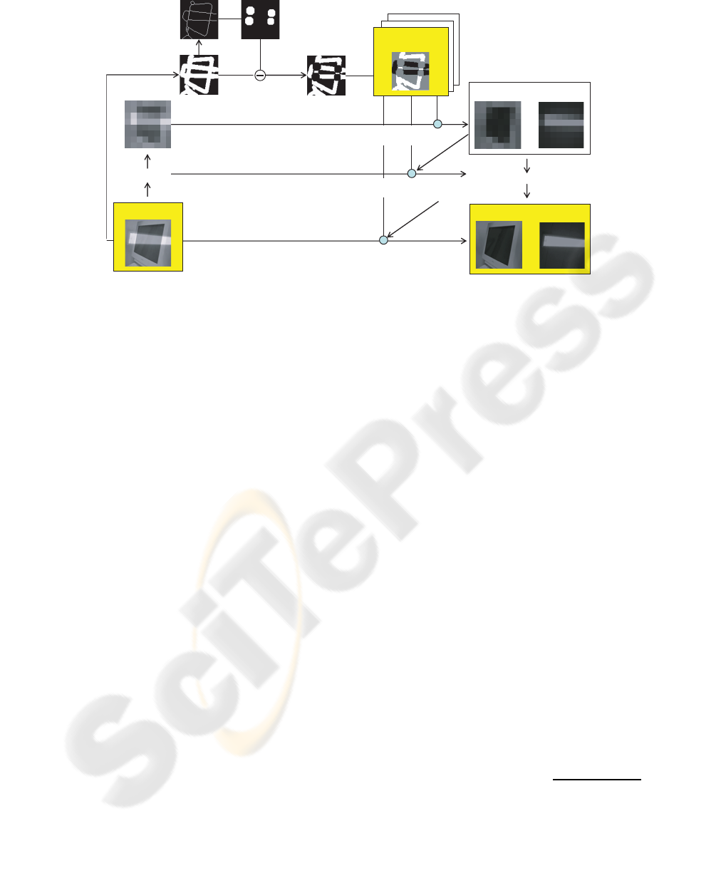
(8) low resolution layers
(1) input image
(6) classified edges
(2) edges
(3) thinned edges
(4) crossing edges
(5) edges belonging
to either layer
(7) low resolution image
(9) original resolution layers
decomposition
decomposition
decomposition
Figure 1: Pipeline of reflection separation.
overlap with any edge of another layer, and (3) the
junction edge in the superposition image arises from
the crossing between an edge of a layer and an edge
of another layer.
We first identify each edge pixel in the input im-
age to which layer it belongs using only low level
image features. We then formulate the problem of
decomposing the single image into two layer images
as an optimization problem easier to solve based on
this classification. We show that this optimization
can be approximately solved using a pyramid struc-
ture and deterministic annealing (Geiger and Girosi,
1991; Urahama and Nagao, 1995; Ueda and Nakano,
1998).
2 PROBLEM FORMULATION
Recently, Levin et al. proposed an optimization
frameworkfor separating reflections from a single im-
age (Levin et al., 2004a). They formulated the prob-
lem of decomposing the single superimposed image
I = [I(x, y)] ∈ R
D
into two layers I
1
= [I
1
(x, y)] ∈ R
D
and I
2
= [I
2
(x, y)] = [I(x, y) − I
1
(x, y)] ∈ R
D
, where
D is the input image domain, as minimizing the cost
function:
cost
1
(I
1
, I
2
) = cost
1
(I
1
) + cost
1
(I
2
), (1)
where cost
1
(I
1
) is the total amount of edges and cor-
ners of I
1
:
cost
1
(I
1
) =
∑
(x, y)∈D
|∇I
1
(x, y)|
α
+ ηc(x, y;I
1
)
β
, (2)
where ∇ is the gradient edge operator and c(·) is the
Harris-like corner operator. Also, α, β, and η are set
to 0.7, 0.25, and 15, respectively, which are obtained
from the histgrams of the operators in natural im-
ages (Levin et al., 2002). They provided solutions for
the problem by dividing the image into overlapping
patches and then selecting the optimal set of patches
from a database of natural image patches.
In the approach mentioned above, the problem of
separating reflections using a single image without
such training data or user intervention have not been
tackled. In this section, to address this difficulty, we
will provide an optimization framework.
2.1 Automatic Classification of Edges
In our work, we first estimate to which layer each
edge pixel in the input superimposed image belongs
according to the following procedure.
1. Detect edges
We detect edges in the input image with the SU-
SAN edge detector (Smith and Brady, 1997) (see
also Figure 1 (1))
n(x
0
, y
0
; I, t) =
∑
(x,y)∈D
c(x, y, x
0
, y
0
; I, t) , (3)
c(x, y, x
0
, y
0
; I, t) = 1− exp
−
I(x, y) − I(x
0
, y
0
)
t
6
(4)
where I(x
0
, y
0
) is the intensity value at the pixel
position (x
0
, y
0
) of the input image I and t is the
edge difference threshold parameter. We hereafter
denote by E the set of edge pixels.
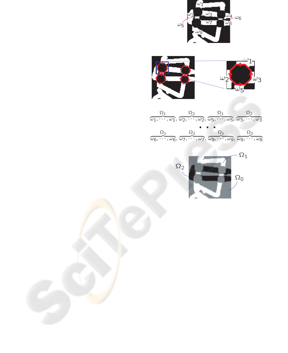
2. Extract edges belonging to either layer
We obtain the set of connected regions, C =
{C
i
|1 ≤ i ≤ m}, by first reducing edges to unit
thickness while maintaining its topology (Fig-
ure 1(2)) and then performing morphological di-
lation of each pixel lying on the intersection of
the two lines with a circular structuring element
of appropriate size (Figure 1(3)). A region which
is C subtracted from the region E can be regarded
as belonging to either layer and can be segmented
into regions ω = {ω
j
|1 ≤ j ≤ n}, where each ω
j
is a connected region and ω
j
∩ ω
k
= φ for j 6= k
and n is the number of ω
j
(Figure 1(4) and Fig-
ure 2(a)).
3. Identify for each edge to which layer it belongs
While tracking around the pixels in the outer
boundary of each C
i
, we sequentially assign a la-
bel to each pixel indicating to which ω
j
it belongs
(no label is assigned to the pixel belonging to none
of ω
j
) (Figure 2(b)). In this process, four kinds of
labels j
1
, j
2
, j
3
, j
4
will appear (Figure 2(c)). Then,
we can impose the constraint that two regions ω
j
1
and ω
j
3
(also, ω
j
2
and ω
j
4
) belong to the same
layer. Hence, we can classify each edge region to
which layer it belongs by solving a set of the con-
straints for all C
i
∈ C (Figure 1(5)). We denote by
Ω
1
, Ω
2
, and Ω
0
the edge region of the first layer,
the edge region of the second layer, and the other
region, respectively (Figure 2(d)).
2.2 Definition of Objective Function
We formulate the problem of separating reflections
from a single image. To make the presentation easy
to read without loss of generality, we will describe
I
1
and I
2
as I
1
= [I
1
(x, y)] = [α(x, y)I(x, y)] ∈ R
D
and
I
2
= [I
2
(x, y)] = [(1 − α(x, y))I(x, y)] ∈ R
D
, respec-
tively, by introducing the set of unknown coefficients,
α = [α(x, y)] ∈ [0, 1]
D
. Then, the task of separating
two transparent layers becomes solving the minimiza-
tion problem as follows.
min
α
f(α; I, t) ≡ min
α
∑
(x, y)∈D
w
1
(x, y)n(x, y; α∗ I, t)
+w
2
(x, y)n(x, y; (E − α) ∗ I, t), (5)
where α ∗ I = [α(x, y)I(x, y)] ∈ R
D
, (E − α) ∗ I =
[(1− α(x, y))I(x, y)] ∈ R
D
, n(x, y; I, t) is the function
defined by Equation (4), w
1
= [w
1
(x, y)] ∈ R
D
and
w
2
= [w
2
(x, y)] ∈ R
D
are the variable weighting func-
tions as
w
1
(x, y) =
w
normal
(x, y) ∈ Ω
0
w
small
(x, y) ∈ Ω
1
w
large
(x, y) ∈ Ω
2
,
(6)
(b)
(c)
(d)
(a)
Figure 2: Classifying each edge according to the layer it
belongs to.
w
2
(x, y) =
w
normal
(x, y) ∈ Ω
0
w
large
(x, y) ∈ Ω
1
w
small
(x, y) ∈ Ω
2
,
(7)
where w
normal
= 1.0, w
large
= 10.0Cw
small
= 0.1. For
a relatively small region of Ω
1
∪ Ω
2
(for a relatively
large region of Ω
0
), the cost function in Equation (5)
becomes multimodal and there are local minima.
2.3 Heuristic Minimization
Next, we consider to employ a simple local search
strategy with a steepest descent heuristic to solve
the nonlinear problem of solving Equation (5). This
consists of setting the initial state of α, select-
ing a pixel with coordinates (x, y) at random, and
then replacing the value of α(x, y) at the current
time step by the neighboring solution that minimizes
Equation (5) within the neighborhood {α(x, y) −
δ, α(x, y), α(x, y) + δ} ; if a solution with no improv-
ing neighbor has been reached, the above heuristic
stops, and otherwise it is iterated.
Although the objective function in Equation (5)
appears to be easier to minimize than the objective
function in Equation (1), Equation (5) also still has
high multimodality and high dimensionality, and thus
the above local search often leads to local minima in
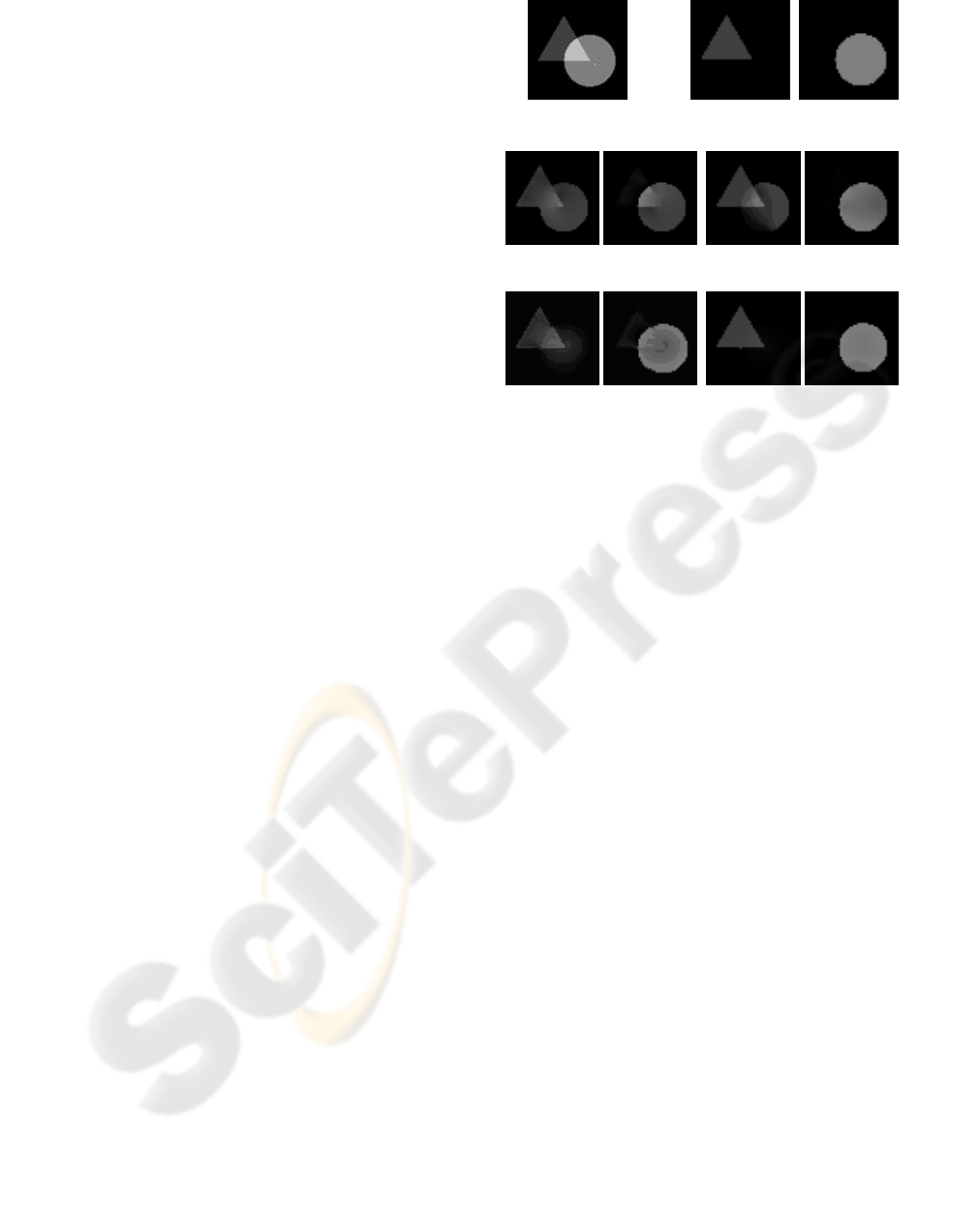
the search space. Examples of the results obtained
using this approach are shown in Figure 3 on a very
simple synthetic image. Figure 3(a) and Figure 3(b)
show the input superimposed image and the ground
truth layers, respectively. Figure 3(c) shows the re-
sult obtained using the local search described in this
section. Figure 3(d) shows another result where the
edge classification described in Section 2.1 was not
utilized. These results show that even though the edge
classification can improve the performance, this com-
plex nonlinear optimization problem in Equation (5)
cannot be solved in any way directly using the sim-
ple heuristic described above. To solve Equation (5),
we can apply powerful deterministic annealing tech-
niques as we will see in the next section.
3 IMAGE DECOMPOSITION
The output of the SUSAN edge detector ranges from
0 (non-edge) to 1 (edge). In Figure 4, each horizon-
tal bar in the graph represents the values of the SU-
SAN edge detector, n(x, y; I, t), for a fixed t, with re-
spect to variation of the gradient magnitude of pixel
at position (x, y). One can see that large t makes the
SUSAN edge detector less sensitive and thus makes
n(x, y; α∗ I, t) and n(x, y; (E − α) ∗ I, t ) in Equation
(5) more uniform over the xy-plane. Also, the lower
the space frequency of the input image I is, the more
uniform n(x, y; α∗ I, t) and n(x, y; (E − α) ∗ I, t ) will
become. In this way, the number of local minima
of the objective function (5) decreases monotonically
with increasing t and smoothed image I.
Based on the above observation, in our frame-
work, we solve Equation (5) using a pyramid struc-
ture and deterministic annealing (Geiger and Girosi,
1991; Urahama and Nagao, 1995; Ueda and Nakano,
1998). After building a multiresolution image pyra-
mid from the input image, we start decomposing the
low resolution image into two images. Until the high-
est resolution (original image), the solution is prop-
agated to the next higher resolution where it is used
as the initial estimate. At each resolution level, the
deterministic annealing is performed by initially set-
ting t to a sufficient large value and then gradually de-
(a) (b)
(c) (d)
(e) (f)
Figure 3: Importance of edge classification and annealing.
(a) Input image. (b) Ground truth images. (c) Without edge
classification and without annealing. (d) With edge classi-
fication and without annealing. (e) Without edge classifi-
cation and with annealing. (f) With edge classification and
with annealing.
creasing it after each iteration, as shown in Figure 5.
The whole procedure of our algorithm is described in
detail below.
1. Extract edges from the input image (I) and clas-
sify each edge to which layer it belongs (Sec-
tion 2.1).
2. Build a pyramid representation of the input image.
In this case, the multiresolution image pyramid
has multiple layers with the original image at the
bottom and compressed (lower spatial resolution)
images at the upper layers. A layer pixel has the
value averaged over the corresponding next lower
(higher spatial resolution) layer four pixels. In this
paper, we choose the number of pyramid layers as
2.
3. Set the current layer to the top most layer and
initialize the separation coefficients (α) such that
α(x, y) = 0.5 for all (x, y) ∈ D.
4. Decompose the current layer image into two im-
ages. In this case, if the current layer is the top
most layer, the initial values of α are set as spec-
ified above, otherwise are set such that the esti-
mated value of α(x, y) of the next upper layer is
mapped to the corresponding four pixels of the
current layer, for all (x, y). Then, decompose the
current layer image according to the following an-
nealing procedure (steps (a) to (c)).
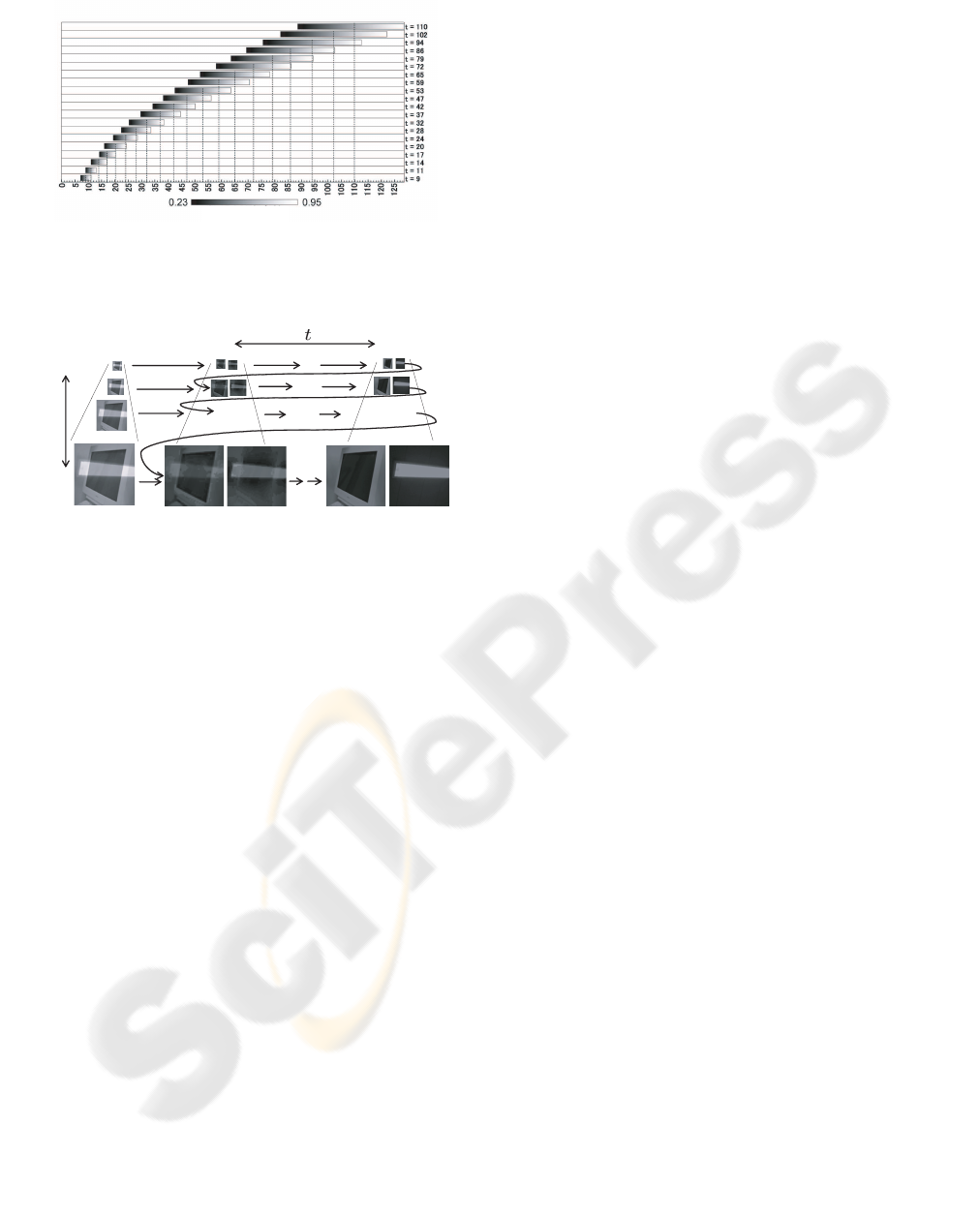
Figure 4: Edge detection sensibility with respect to varia-
tions of t. The horizontal and vertical axes represent the
gradient magnitude and t, respectively.
resolution
large
small
low
high
Figure 5: Reflection separation with a pyramid structure and
deterministic annealing.
(a) Initially set the edge difference threshold para-
meter (t) of the SUSAN edge detector to a large
value.
(b) Compute α under the current layer and t value
using the heuristic minimization (Section 2.3).
(c) Iterate between decreasing t and the above step
(b) until t reaches its destination.
5. Iterate between moving to the next lower layer
and finding the best composition under this layer
(step. 4) until the bottom layer (the original im-
age) is reached.
6. If multiple edge classifications are possible
(Section 2.1), perform the image decomposition
(steps 1 to 5) for each classification and then
select the decomposition result which solves
Equation (5) in the case where Ω
1
∪ Ω
2
= φ,
i.e., w
1
(x, y) = w
2
(x, y) = w
normal
for all pixel
(x, y) ∈ D.
Figures 3(e), (f) show the decomposition results
obtained using deterministic annealing with and with-
out edge classification, respectively. One can see that
good decomposition results cannot be obtained with-
out using edge classification. Although deterministic
annealing offers no theoretical guarantee of finding
the global optimum, it is well known that it can avoid
many local minima (Geiger and Girosi, 1991; Ura-
hama and Nagao, 1995; Ueda and Nakano, 1998).
4 RESULTS
To demonstrate and evaluate our method, we used
real and synthetic images as inputs. First, we pho-
tographed a doll behind a glass window which was
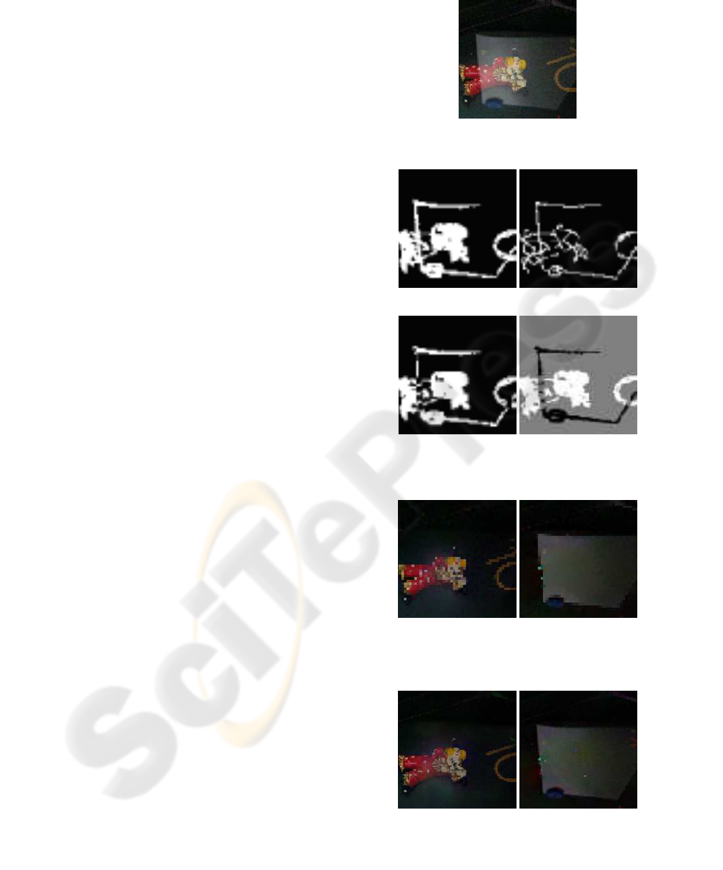
reflected by the glass. Figure 6 shows the input image
(100x100 pixels). We extracted edges using the SU-
SAN edge detector (Figure 7(a)), thinned the edges
(Figure 7(b)), eliminated the crossing edges (Fig-
ure 7(c)) and classified each edge to which layer it
belongs (Figure 7(d)), as described in Section 2.1.
Using the estimated classification of edges, we con-
structed an image pyramid from the input image and
decomposed the top most layer, as shown in Figure 8.
As shown in Figure 9, using this decomposition re-
sult as an initial guess, we decomposed the original
image into two images. This appears to be a quali-
tatively good result. In this case, we processed each
RGB channel separately.
Next, in order to evaluate the results of our method
quantitatively against ground truth, we used as input
the generated image by summing two already cap-
tured or synthetic images. Figures 10– 14 show the
input images, corresponding ground truth decompo-
sitions, and resulting decompositions. Figures 10 and
11 showexamples of using as inputs the generated im-
ages by summing two relatively simple images. One
can see that quite good results were obtained. Fig-
ures 12 and 13 show examples of using as inputs the
addition of simple and complex images. Despite some
undesired ghost images such as the baby’s face in Fig-
ure 12(c) and highlight in Figure 13(c), fairly good re-
sults seem to be obtained. Figure 14 shows an exam-
ple of using as an input the generated image by sum-
ming two relatively complex images. In Figure 14(c)
one can see several ghost images. The decomposition
algorithm roughly took about 15 minutes on a single
Pentium IV 2.4GHz processor.
Again, for the purpose of verifying the effec-
tiveness of the edge classification described in Sec-
tion 2.1, we separated the input images in Fig-
ures 11(a), 13(a) without classifying edges, as at-
tempted in Figure 3(e). In both of these examples,
the image decomposition failed due to convergence at
local minima, as shown in Figure 15(a), (b). Those
examples demonstrate the significance of classifying
edges for separating.
5 CONCLUSIONS
We proposed a novel method for decomposing a sin-
gle superimposed image into two images. Despite us-
ing neither image database nor user intervention, we
showed that the almost fully automatic layer extrac-
tion can be achieved using only a single input im-
age. One of the research problems to be solved in our
method is to provide robustness to errors in the edge
detection and classification. We are currently study-
ing to adapt the different error recovery schemes.
REFERENCES
Farid, H. and Adelson, E. H. (1999). Separating reflec-
tions from images by use of independent components
analysis. JOSA, vol.16, no.9, pp.2136–2145.
Geiger, D. and Girosi, F. (1991). Parallel and deterministic
algorithms from mrf’s: Surface reconstruction. IEEE
PAMI, vol.13, no.5, pp.401–412.
Irani, M. and Peleg, S. (1992). Image sequence enhance-
ment using multiple motions analysis. Proc. IEEE
CVPR, pp.216–221.
Levin, A., Zomet, A., and Weiss, Y. (2002). Learning
to perceive transparency from the statistics of natural
scenes. IEEE NIPS.
Levin, A., Zomet, A., and Weiss, Y. (2004a). Separating
reflections from a single image using local features.
Proc. IEEE CVPR, pp.306–313.
Levin, A., Zomet, A., and Weiss, Y. (2004b). User assisted
separation of reflections from a single image using a
sparsity prior. Proc. ECCV, pp.602–613.
Sarel, B. and Irani, M. (2004a). Separating transparent lay-
ers of repetitive dynamic behaviors. Proc. IEEE ICCV,
pp.26–32.
Sarel, B. and Irani, M. (2004b). Separating transparent lay-
ers through layer information exchange. Proc. ECCV,
pp.328–341.
Schechner, Y., Shamir, J., and Kiryati, N. (2000). Blind re-
covery of transparent and semireflected scenes. Proc.
IEEE CVPR, pp.1038–1043.
Smith, S. M. and Brady, M. (1997). Susan -a new approach
to low level image processing. IJCV, vol.23, no.1,
pp.45–78.
Szeliski, R., Avidan, S., and Anandan, P. (2000). Layer
extraction from multiple images containing reflections
and transparency. Proc. IEEE CVPR.
Tsin, Y., Kang, S. B., and Szeliski, R. (2003). Stereo match-
ing with reflections and translucency. Proc. IEEE
CVPR, pp.702–709.
Ueda, N. and Nakano, R. (1998). Deterministic annealing
em algorithm. Neural Networks, vol.11, no.2, pp.272–
282.
Urahama, K. and Nagao, T. (1995). Direct analog rank fil-
tering. IEEE Trans. Circuits Syst. I, vol.42, pp.385–
388.
Figure 6: Input image.
(a) (b)
(c) (d)
Figure 7: Edge detection and classification.
Figure 8: Intermediate result (decomposition on low reso-
lution image).
Figure 9: Decomposition.
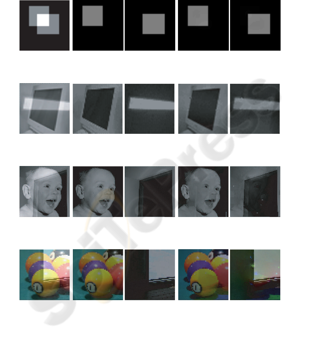
(a) (b) (c)
Figure 10: Result. (a) Input image (synthesized by summing the simple images in b). (b) Ground truth images. (c) Decompo-
sition.
(a) (b) (c)
Figure 11: Result. (a) Input image (synthesized by summing the simple images in b). (b) Ground truth images. (c) Decompo-
sition.
(a) (b) (c)
Figure 12: Result. (a) Input image (synthesized by summing the complex and simple images in b). (b) Ground truth images.
(c) Decomposition.
(a) (b) (c)
Figure 13: Result. (a) Input image (synthesized by summing the complex and simple images in b). (b) Ground truth images.
(c) Decomposition.
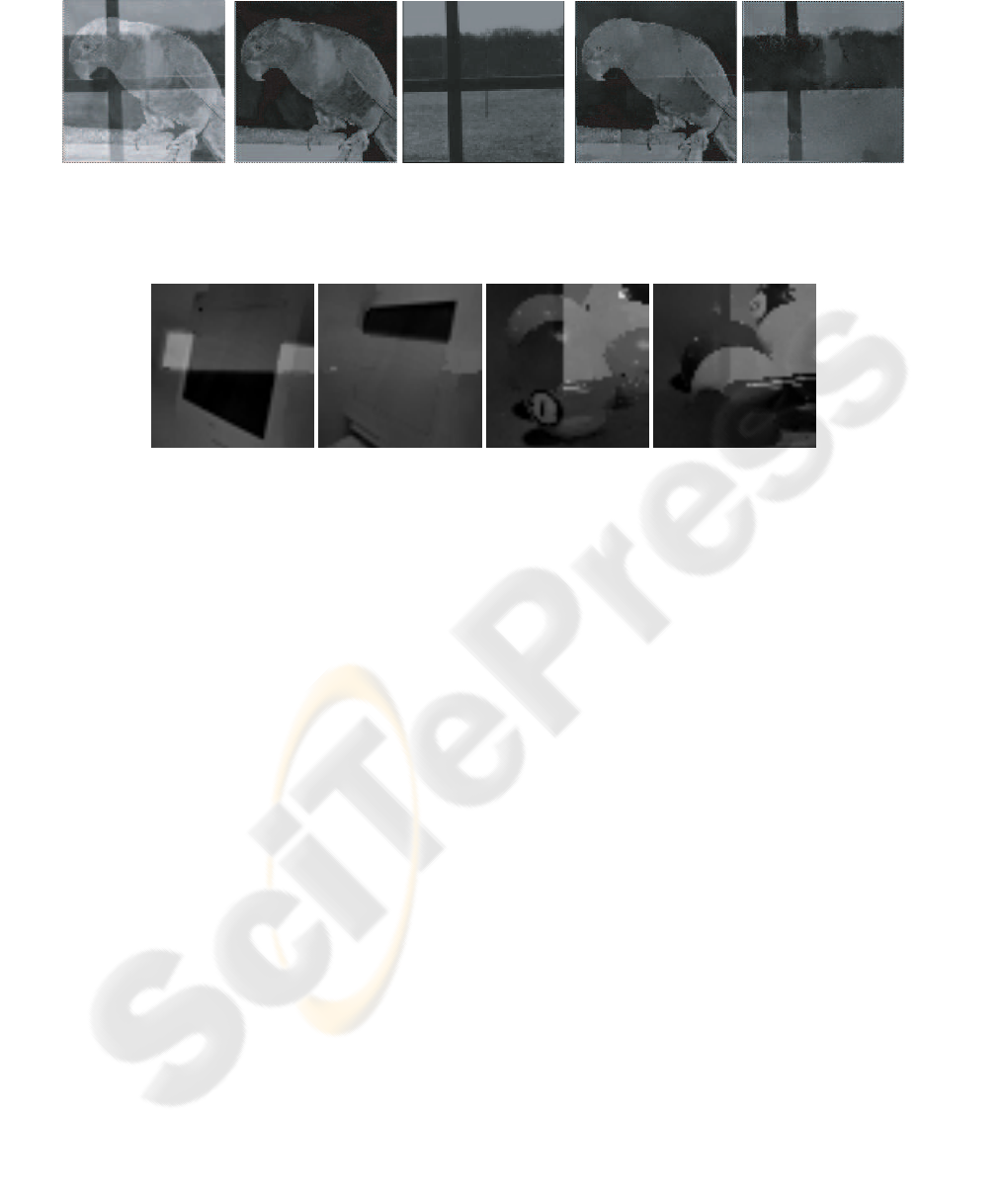
(a) (b) (c)
Figure 14: Result. (a) Input image (synthesized by summing the complex images in b). (b) Ground truth images. (c)
Decomposition.
(a) (b)
Figure 15: Results without classifying edges. (a) Decomposition when the image of Fig. 11(a) is taken as an input. (b)
Decomposition when the separated green channel image of the image of Fig. 13(a) is taken as an input.
