
A CLOSED-FORM SOLUTION FOR THE GENERIC
SELF-CALIBRATION OF CENTRAL CAMERAS
FROM TWO ROTATIONAL FLOWS
Ferran Espuny
Departament d’
`
Algebra i Geometria, Universitat de Barcelona, Spain
Keywords:
Self-calibration, generic camera, non-parametric sensor, optical flow.
Abstract:
In this paper we address the problem of self-calibrating a differentiable generic camera from two rotational
flows defined on an open set of the image. Such a camera model can be used for any central smooth imaging
system, and thus any given method for the generic model can be applied to many different vision systems.
We give a theoretical closed-form solution to the problem, proving that the ambiguity in the obtained solution
is metric (up to an orthogonal linear transformation). Based in the theoretical results, we contribute with an
algorithm to achieve metric self-calibration of any central generic camera using two optical flows observed in
(part of) the image, which correspond to two infinitesimal rotations of the camera.
1 INTRODUCTION
The first proposed generic camera model consisted of
a finite set of pixels and imaging rays in a one-to-
one correspondence; its calibration-from-pattern was
already solved in a quite pleasant way (Sturm and
Ramalingam, 2004; Grossberg and Nayar, 2001), al-
though some questions remain open. This model can
be used for any vision system with little assumption,
in contrast with the classical approaches that impose
a parametric restriction to estimate a model (Hartley
and Zisserman, 2000).
In (Ramalingan et al., 2005) a first metric
self-calibration (calibration without scene o motion
knowledge) algorithm was presented from at least two
rotations and one translation of a generic central cam-
era, i.e. with a single effective viewpoint. The authors
explicitly admitted that the model should be changed
to a continuous one with infinitely many rays.
We consider the continuous (resp. differentiable)
generic central camera model to be described by a
continuous (resp. differentiable) bijective map ϕ be-
tween an sphere and the image plane. An image is
obtained by composing the central projection on the
sphere (the ideal central camera) with this warping
map from the sphere onto the image plane. Note that
ϕ gives us a one-to-one correspondence between im-
age points and projection rays, and thus our definition
is consistent with the discrete generic camera model.
The differentiable model was introduced in
(Nist
´
er et al., 2005), where a closed-form formula
was given for the projective self-calibration (i.e. re-
covering ϕ up to projective ambiguity) from at least
three observed optical flows corresponding to three
infinitesimal rotations. In (Grossmann et al., 2006), a
first method for metric self-calibration from only two
rotational flows was given. The method gave a ex-
perimentally unique solution, which was shown to be
extremely sensitive to noise and even to fail with cer-
tain exact simulated flows.
We give a theoretical closed-form solution to the
problem of self-calibrating a differentiable generic
camera from two rotational flows defined on an open
set of the image. We also proof that the solution is
unique up to an orthogonal linear transformation. Our
main contribution is an algorithm to achieve metric
self-calibration of any central smooth imaging sys-
tem using two optical flows observed in (part of) the
image, which correspond to two linearly independent
rotations. We use simulated data to show that the
proposed method performs well with both exact and
noisy optical flows.
26
Espuny F. (2007).
A CLOSED-FORM SOLUTION FOR THE GENERIC SELF-CALIBRATION OF CENTRAL CAMERAS FROM TWO ROTATIONAL FLOWS.
In Proceedings of the Second International Conference on Computer Vision Theory and Applications - IFP/IA, pages 26-31
Copyright
c
SciTePress
2 PROBLEM FORMULATION
2.1 Differentiable Generic Camera
We will describe the calibration of a general central
camera by a regular 2-differentiable map f between
the image plane and the unit sphere:
f : R
2
→ S
2
(u,v) 7→ f(u,v).
(1)
We take as ideal central camera the standard spherical
projection
π : R
3
→ S
2
p 7→ p/kpk.
(2)
According to (Nist
´
er et al., 2005) we model any
central camera as the composition of π with ϕ =
f
−1
, which warps the spherical image onto the im-
age plane. Note that the calibration map f gives us
a locally one-to-one correspondence between image
points and projection rays, agreeing with the calibra-
tion concept introduced by (Sturm and Ramalingam,
2004) for the (discrete) generic camera model.
2.2 Self-Calibration Problem
We assume that we know on the image two 2-
differentiable optical flows
v
i
: R
2
→ R
2
(u,v) 7→ v
i
(u,v) ,
(3)
both defined on a common open subset. We also
suppose that the observed flows v
i
correspond to in-
finitesimal rotations of the camera with respective
(unknown) linearly independent angular velocities ω
i
.
Our problem consists in determining the possible
angular velocities ω
i
and calibration map f that are
compatible with the image flows v
i
.
Since each infinitesimal Euclidean rotation with
angular velocity ω
i
induces on the unit sphere a tan-
gent vector field defined by
p ∈ S
2
7→ ω
i
∧ p ∈T
p
S
2
, (4)
following (Nist
´
er et al., 2005) the problem can be for-
mulated as that of finding f and ω
i
, i = 1,2, such that
Df(u,v) ·v
i
(u,v) = ω
i
∧ f(u,v) , (5)
being Df = ( f
u
|f
v
) the 3×2 differential matrix of f.
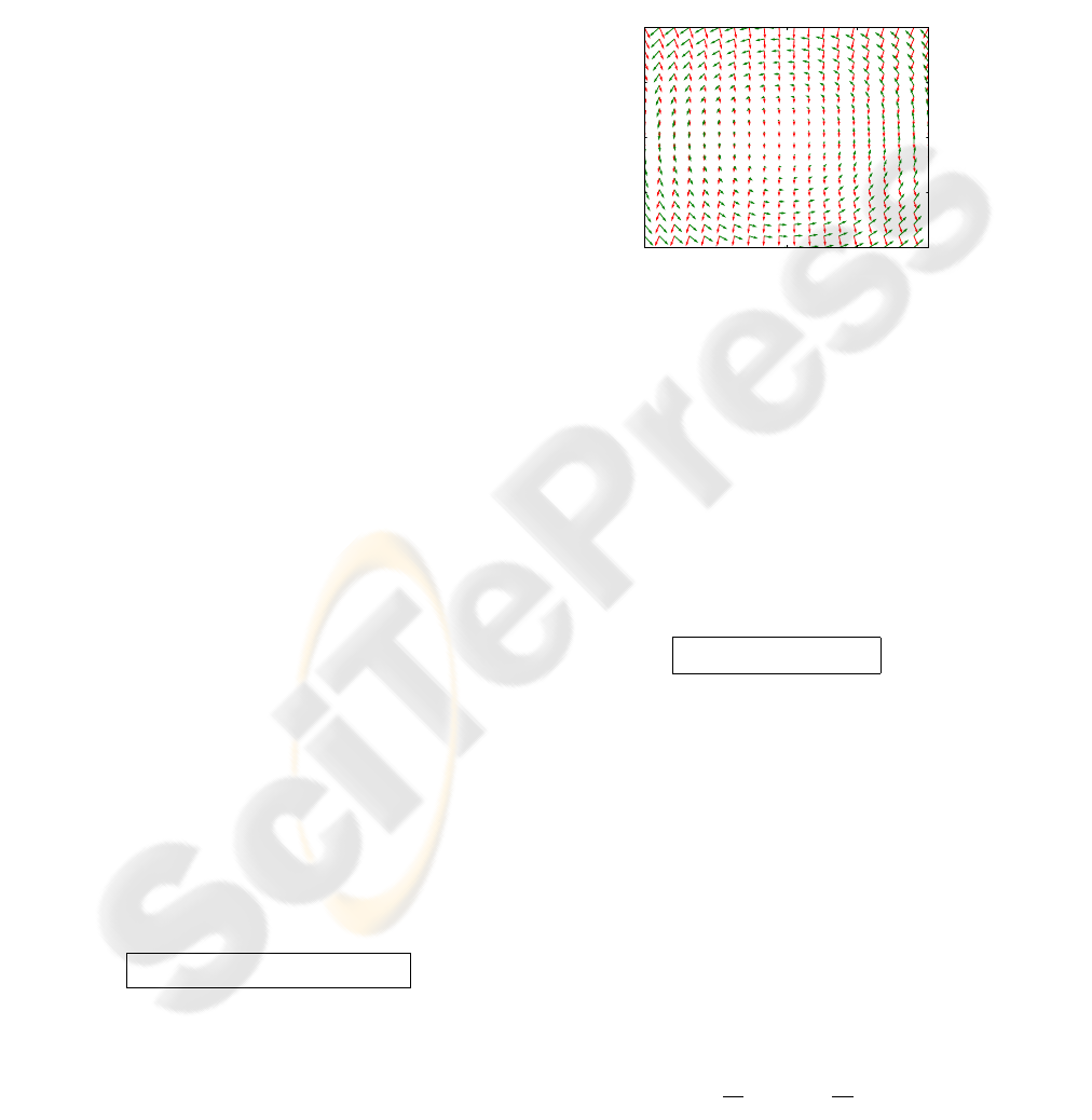
Observe that, although the rotation axes are re-
quired to be linearly independent, the induced flows
on the sphere will always be linearly dependent along
a circle (see Figure 1). Therefore, when this circle is
mapped by f
−1
on an image curve, the optical flows
will be linearly dependent along that set of points.
Thus, we restrict ourselves to solve (5) for those
points (u,v) in an open connected subset of image
points where the optical flows are linearly indepen-
dent. Once we have determined f on the open con-
nected subsets with independent flows, it can be ex-
tended by continuity to the whole image.
-1.0 -0.5 0.0 0.5 1.0
-1.0
-0.5
0.0
0.5
1.0
Spherical Flows Projected on {z=1}
Figure 1: Projection on the plane {z = 1} of two spherical
flows, with angular velocities ω
1
= (1, 0, 0) (going down)
and ω
2
= (0,0,1) (rotating anti-clockwise). The projected
flows are linearly dependent along the line {y = 0}, which
corresponds to a circle through the flow singular points.
2.3 Notations
We define the 2 × 2 matrix V := (v
1
|v
2
), and take
˜
V := V
−1
=
˜v
11
˜v
21
˜v
12
˜v
22
, where it exists. Observe
that, with these notations, equation (5) says
Df = −[ f]
×
(ω
1
|ω
2
)
˜
V . (6)
For any differentiable function ϕ : R
2
→ R
m
we
denote by Dϕ = (ϕ
u
|ϕ
v
) its m×2 differential matrix.
3 A CLOSED-FORM SOLUTION
3.1 Theoretical Results
For a given flow matrix V we want to determine the
possible f and ω
i
’s satisfying the matrix equation (6).
First we show that we can reduce the problem to that
of determining the angular velocities ω
i
.
Let
˜
∆ = (
˜
∆
1
,
˜
∆
2
) be the vector function defined by
˜
∆
1
˜
∆
2
:=
∂
∂v
˜v
11
˜v
12
−
∂
∂u
˜v
21
˜v
22
. (7)

Theorem 1. Assume that we know ω
1
and ω
2
, the an-
gular velocities of the infinitesimal rotation motions.
We consider
˜g :=
˜
∆
1
ω
1
+
˜
∆
2
ω
2
+ det
˜
Vω
1
∧ω
2
6= 0 , (8)
Then, the calibration map f can be computed as
f = ±
˜g
k˜gk
.
Proof. If we know ω
1
and ω
2
we can compute the
following 3×2 functions:
a := (ω
1
|ω
2
)
˜v
11
˜v
12
, b := (ω
1
|ω
2
)
˜v
21
˜v
22
. (9)
By (6), we are looking for f such that
f
u
= [a]
×
f ,
f
v
= [b]
×
f .
(10)
Since f is 2-differentiable, it must hold
0 = f
uv
− f
vu
= ( f
u
)
v
−( f
v
)
u
(10)
= [a
v
]
×
f + [a]
×
f
v
−[b
u
]
×
f −[b]
×
f
u
(10)
= [a
v
−b
u
]
×
f + ([a]
×
[b]
×
−[b]
×
[a]
×
) f
= [a
v
−b
u
+ a∧b]
×
f
(8)
= [ ˜g]
×
f ,
from what it follows that f and ˜g must be propor-
tional. Observe that, since the vectors ω
1
, ω
2
and
ω
1
∧ω
2
form a basis of R
3
, and det
˜
V 6= 0, the function
˜g never vanishes. Finally, the result can be obtained
by imposing kfk= 1.
Remark 1. In order to improve the stability of the nu-
merical computation of f , we will use the formula
f = ±g/kgk, with g = (detV ˜g) expressed as follows:
g = ∆
1
ω
1
+ ∆
2
ω
2
+ ω
1
∧ω
2
, (11)
where ∆ = (∆
1
,∆
2
) is given by
∆
1
∆
2
:=
∂v
21
∂u
+
∂v
22
∂v
−
detV
u
detV
v
21
−
detV
v
detV
v
22
−
∂v
11
∂u
−
∂v
12
∂v
+
detV
u
detV
v
11
+
detV
v
detV
v
12
.
(12)
Next we give a closed-form formula to find ω
i
, the
rotation flow angular velocities, using only the image
flows v
i
. We also determine the ambiguity in the given
solution.
Theorem 2. The matrix G
ω
:= (ω
1
|ω
2
)
t
(ω
1
|ω
2
) can
be determined from V using the formula
G
ω
=
∆
2
−∆
1
(−∆
2
|∆
1
) −
D∆
2
−D∆
1
V . (13)
Thus, given V the angular velocities ω
i
can be de-
termined up to an orthogonal transformation of the
Euclidean space R
3
.
Proof. By imposing (6) to the function f = ±
g
kgk
,
where g is defined in (11), we obtain (note that the
sign ambiguity cancels out in both sides):
−
g
kgk
×
(ω
1
|ω
2
)V
−1
= D(
g
kgk
)
= gD(
1
kgk
) +
1
kgk
Dg
= −
1
kgk
(g
g
t
Dg
g
t
g
−Dg) ,
where in the last step we have used that kgk =
√
g
t
g.
Thus, taking A :=
g
t
Dg
g
t
g
, we have obtained the follow-
ing relation:
[g]
×
(ω
1
|ω
2
) = (gA−Dg)V . (14)
By (11) the left-hand side term in (14) is
[∆
1
ω
1
+ ∆
2
ω
2
]
×
(ω
1
|ω
2
) +[ω
1
∧ω
2
]
×
(ω
1
|ω
2
) ,
which can be simplified as
ω
1
∧ω
2
(−∆
2
|∆
1
) +(ω
1
|ω
2
)
0 −1
1 0
G
ω
. (15)
Now, (14) can be decomposed in two equalities. The
first one corresponds to the components on the direc-
tion of ω
1
∧ω
2
: (−∆
2
|∆
1
) = A V, which gives us
A = (−∆
2
|∆
1
)V
−1
. (16)
A second equality can be obtained by comparing the
parts in (14) on the plane generated by ω
1
and ω
2
:
0 1
−1 0
G
ω
= (∆ A−D∆)V . (17)
The formula for G
ω
in the Theorem follows from this
last equality using (16). Since we can only know the
norm and scalar product of the ω
i
, they are determined
up to an orthogonal transformation M ∈ O(R
3
). Ob-
serve that the remaining ambiguity is inherent to the
problem: if f and ω
i
satisfy (5), then M f and Mω
i
also give a solution.
3.2 Self-Calibration Algorithm
Assume that we know two optical flows v
1
, v
2
defined
on the whole image, corresponding to two infinitesi-
mal rotations of unknown angular velocities ω
1
, ω
2
.
We fix two directions d
1
,d
2
∈ R
3
, which we will
use to remove the ambiguity in the determination of
the solution.
We propose the following algorithm:
1) Compute ε(u, v) a measure of linear dependence
of the flows at each image pixel:
ε :=
det(v
1
|v
2
)
kv
1
k
2
+ kv
2
k
2
. (18)
2) Compute the functions ∆
i
(u,v) defined in (12),
and use the formula for G
ω
in (13) to compute
matrices G(u,v) =
A B
1
B
2
C
.
3) Compute
C the set of pixels (u,v) such that:
i) A(u,v) > 0 ,
ii) C(u, v) > 0 ,
iii) |B
1
(u,v) −B
2
(u,v)| < median(|B
1
−B
2
|) ,
iv) (u, v) is not in the border of the image,
v) ε(u,v) > median(ε) .
Using B := (B
1
+ B
2
)/2, take the means of A, B
and C inside C as the coefficients of G
ω
.
4) Compute ω
1
,ω
2
such that ω
1
= λ
1
d
1
and
ω
2
= µ
1
d
1
+ µ
2
d
2
, with λ
1
> 0, µ
2
> 0 and
(ω
1
|ω
2
)
t
(ω
1
|ω
2
) = G
ω
.
5) Take g(u,v) as defined in (11), and finally
f(u,v) := sign(g
3
(u,v))
g
kgk
, (19)
unless fixing f
3
(u,v) > 0 is not convenient.
3.3 Comments
Since in practice we only know the optical flow on a
grid of pixels, the computation of the ∆
i
, which re-
quires first derivatives, and the computation of G
ω
,
involving second derivatives of the flow, will be less
accurate at the borders of the image. Note also that
the error (5) in a few pixels could be big due to the
division in (12); the estimation of f in those pixels
can be improved by imposing the smoothness of f in
a neighborhood containing pixels with lower error.
Besides that, the formula (13) gives us as many
estimators for G
ω
as image points. We select in step
3 those points inside the image where the matrices
are (closer to be) symmetric definite positive and the
optical flows are (closer to be) linearly independent.
Alternative criteria can be used, specially if the sug-
gested conditions turn out to be too restrictive.
Finally, reversing the order in the flows (and ro-
tations) changes the sign of the ∆
i
(u,v) in (12), and
thus the sign of g in (11). Fixing f
3
(u,v) > 0 in step 5
makes the algorithm independent of the flows order.
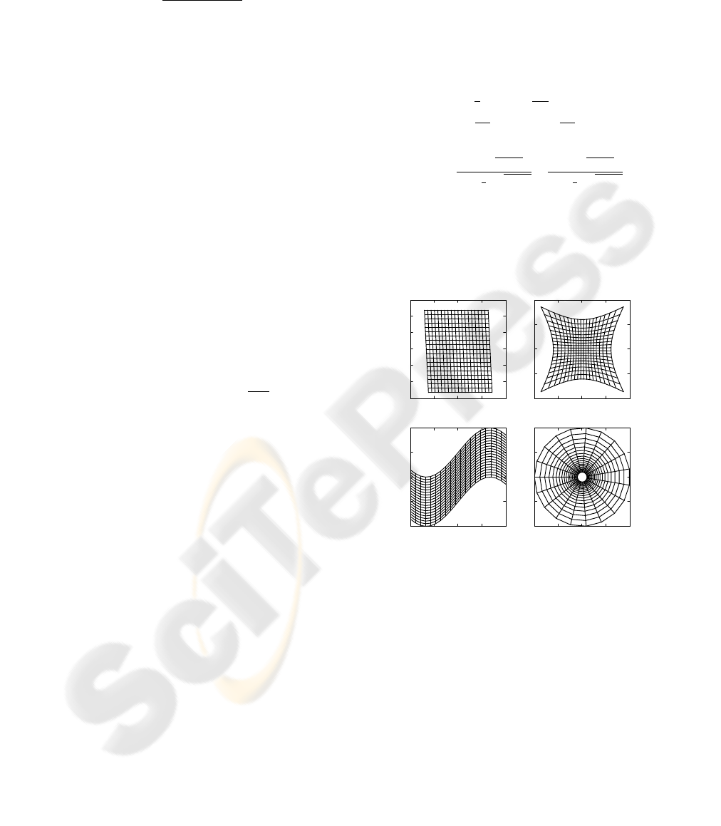
4 EXPERIMENTAL RESULTS
We simulated different generic calibration maps f :
S
2
→ R
2
by composing T : S
2
→ R
2
, the central pro-
jection from the unit sphere onto the plane {z = 1},
with rectifying maps F : R
2
→ R
2
defined on the
plane {z = 1}. We considered different maps (Gross-
mann et al., 2006):
1. F(u,v,1) = K
−1
(u,v,1), pinhole sensor,
2. F(u,v,1) = (u,
1
2
(v+sin(
3πu
4
)),1), sine sensor,
3. F(u,v,1) = (10
u−1
2
cos(πv),10
u−1
2
sin(πv),1), log-
polar sensor,
4. F(u,v) = (
tan(θ
√
u
2
+v
2
)
2tan(
θ
2
)
√
u
2
+v
2
u,
tan(θ
√
u
2
+v
2
)
2tan(
θ
2
)
√
u
2
+v
2
v,1), a
fish-eye model with angular field of view θ (De-
vernay and Faugeras, 2001),
with (u,v) ∈ (−1,1) ×(−1,1). See Figure 2 for a
20×20 discrete representation of the sensors.
-2.0 -1.2 -0.5 0.2 1.0
-1.5
-1.0
-0.5
0.0
0.5
1.0
1.5
Pinhole
-2.0 -1.0 0.0 1.0 2.0
-2.0
-1.0
0.0
1.0
2.0
Fish-eye
-1.0 -0.5 0.0 0.5 1.0
-1.0
-0.5
0.0
0.5
1.0
Sine
-1.0 -0.5 0.0 0.5 1.0
-1.0
-0.5
0.0
0.5
1.0
Log-polar
Figure 2: Examples of the considered ”unwarping” maps f.
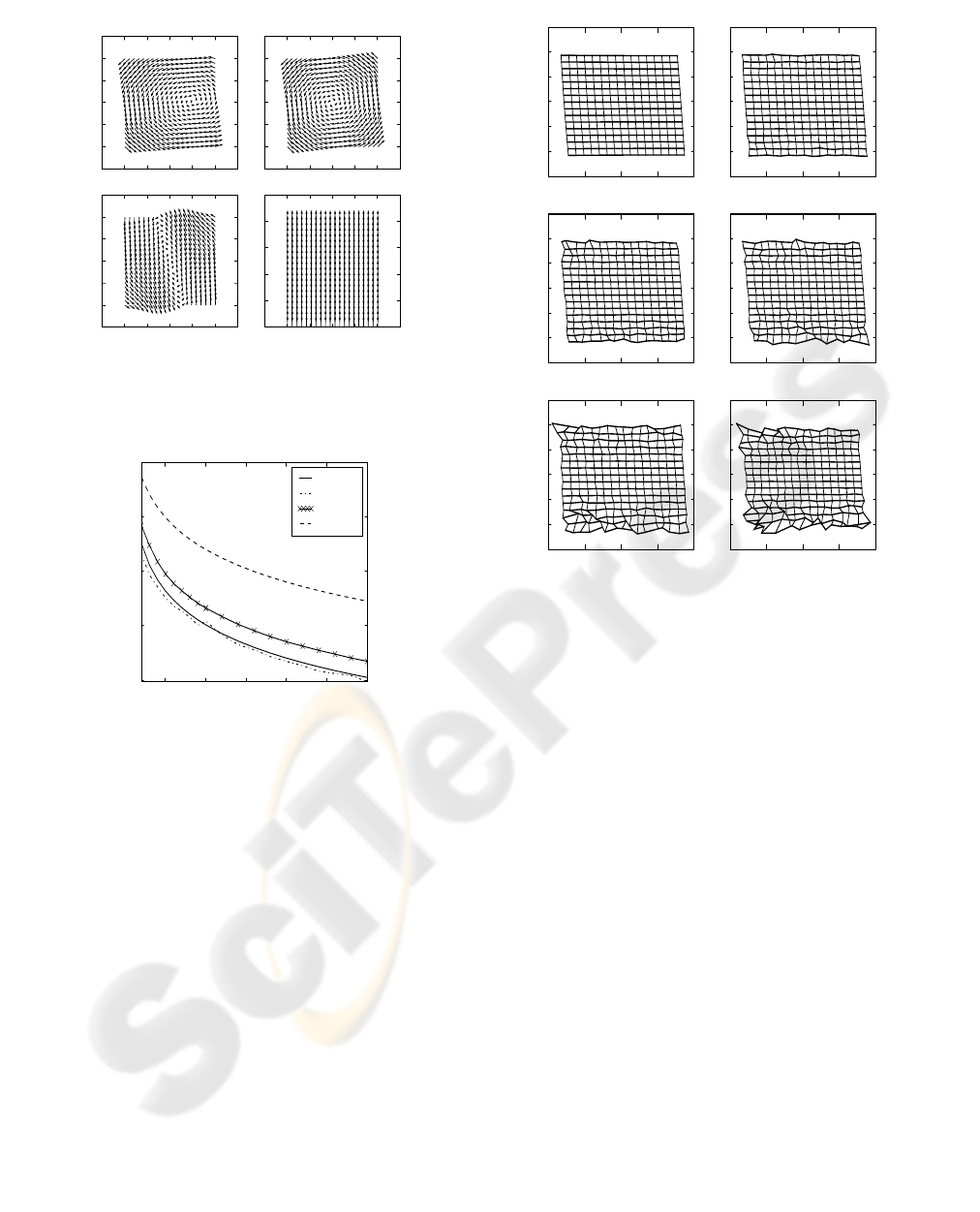
In a first experiment, we wanted to study the be-
havior of Algorithm 3.2 with exact data. For each
sensor, we simulated two optical flows in a 20 ×20
discrete image, like those in Figure 3, and computed
the estimations for G
ω
and f. The goodness of the
obtained f with the Pinhole and Sine models can be
observed in the upper-left picture in figures 5 and 6
respectively, for ω
1
= (0.2,0,0) and ω
2
= (0,0,0.2).
Since our algorithm needs to estimate numerically
the derivatives of the optical flows, it is expected to
work better with very dense flows. The improvement
in the solution with respect to the size of the image
flow grid (taken to have N ×N pixels, with N rang-
ing from 20 to 300) can be observed in Figure 4. We
-1.5 -1.0 -0.5 0.0 0.5 1.0 1.5
-1.5
-1.0
-0.5
0.0
0.5
1.0
1.5
Pinhole
-1.5 -1.0 -0.5 0.0 0.5 1.0 1.5
-1.5
-1.0
-0.5
0.0
0.5
1.0
1.5
Sine
-1.5 -1.0 -0.5 0.0 0.5 1.0 1.5
-1.0
-0.5
0.0
0.5
1.0
1.5
Log-Polar
-1.5 -1.0 -0.5 0.0 0.5 1.0 1.5
-1.5
-1.0
-0.5
0.0
0.5
1.0
1.5
Fish-Eye
Figure 3: Image optical flows with ω = (0,0,0.2).
20 50 100 150 200 250 300
1e-5
1e-4
1e-3
1e-2
1e-1
Flow Error
Pinhole
Fish-Eye
Sine
Log-Polar
Figure 4: Errors with exact data for different image grid
sizes.
used as an over-all error measure the mean of all the
differences in the Flow equation (5).
In a similar way, we varied the field of view in the
Pinhole and Log-Polar sensors, and observed that our
closed-form formulas gave better results with bigger
field of view, i.e. bigger image changes.
In order to simulate real (regular) optical flow
data, we perturbed exact 300×300 image rotational
flows with gaussian noise s relative to the flows (i.e.
v
sim
ij
= (1 + s)v
exact
ij
), then smoothed the flow with a
Gaussian convolution and finally downsampled it into
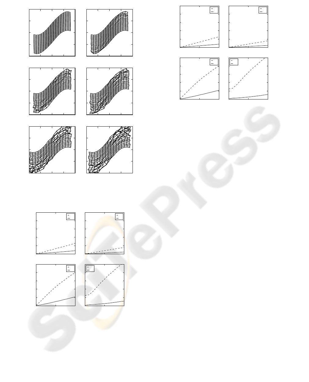
a 20 ×20 flow. In Figures 5 and 6 we show exam-
ples of typical self-calibration results with noise for
ω
1
= (0.2,0,0) and ω
2
= (0,0,0.2).
We observed that, specially in presence of noise,
not only the product matrix G
ω
was important, but
also the initial directions of the ω
i
. As an example,
and to summarize, we show in figures 7 and 8 the be-
-1.5 -1.0 -0.5 0.0 0.5
-1.5
-1.0
-0.5
0.0
0.5
1.0
1.5
s = 0.00
-1.5 -1.0 -0.5 0.0 0.5
-1.5
-1.0
-0.5
0.0
0.5
1.0
1.5
s = 0.01
-1.5 -1.0 -0.5 0.0 0.5
-1.5
-1.0
-0.5
0.0
0.5
1.0
1.5
s = 0.02
-1.5 -1.0 -0.5 0.0 0.5
-1.5
-1.0
-0.5
0.0
0.5
1.0
1.5
s = 0.03
-1.5 -1.0 -0.5 0.0 0.5
-1.5
-1.0
-0.5
0.0
0.5
1.0
1.5
s = 0.04
-1.5 -1.0 -0.5 0.0 0.5
-1.5
-1.0
-0.5
0.0
0.5
1.0
1.5
s = 0.05
Figure 5: Calibration example of the Pinhole sensor with
noise s relative to optical flow; x and z rotation axes.
havior of the considered models with ω
1
= (0.2,0,0)
and either ω
2
= (0, 0.2, 0) or ω
2
= (0, 0, 0.2). Note
that in both cases G
ω
is the same. The relative er-
ror in the estimation of G
ω
(Figure 7) corresponds to
the matrix norm of the difference with its true value
divided by four times the norm of the true matrix.
5 CONCLUSIONS
In this paper we have shown that it is possible to solve
in a closed-form way the problem of self-calibrating
any differentiable generic central camera from only
two rotational flows, not necessarily observed on the
whole image. We have proved that the only remaining
ambiguity in the solution is an orthogonal displace-
ment, which affects both the estimation of the rotation
angular velocities and the calibration map.
We have also given a self-calibration algorithm
based on the previous results. Using simulated data,
we have shown that it works quite well with noisy reg-
ular optical flows, and that its performance improves
with dense image flows and big fields of view. In the
future, strongly encouraged by the obtained results,
-1.0 -0.5 0.0 0.5 1.0
-1.0
-0.5
0.0
0.5
1.0
s = 0.00
-1.0 -0.5 0.0 0.5 1.0
-1.0
-0.5
0.0
0.5
1.0
s = 0.01
-1.0 -0.5 0.0 0.5 1.0
-1.0
-0.5
0.0
0.5
1.0
s = 0.02
-1.0 -0.5 0.0 0.5 1.0
-1.0
-0.5
0.0
0.5
1.0
s = 0.03
-1.0 -0.5 0.0 0.5 1.0
-1.0
-0.5
0.0
0.5
1.0
s = 0.04
-1.0 -0.5 0.0 0.5 1.0
-1.0
-0.5
0.0
0.5
1.0
s = 0.05
Figure 6: Calibration example of the Sine sensor with noise
s relative to optical flow; x and z rotation axes.
0.00 0.05 0.10
0.0
0.1
0.2
0.3
0.4
0.5
Pinhole
xy
xz
0.00 0.05 0.10
0.0
0.1
0.2
0.3
0.4
0.5
Sine
xy
xz
0.00 0.05 0.10
0.0
0.1
0.2
0.3
0.4
0.5
Log-Polar
xy
xz
0.00 0.05 0.10
0.0
0.1
0.2
0.3
0.4
0.5
Fish-Eye
xy
xz
Figure 7: Relative error in G
ω
with respect to noise relative
to the flows; two different rotation pairs are shown.
we will use our algorithm with pairs of real rotational
flows and also adapt it to have a robust self-calibration
method able to work with more than two flows.
0.00 0.05 0.10
0.0
0.1
0.2
0.3
0.4
0.5
Pinhole
xy
xz
0.00 0.05 0.10
0.0
0.1
0.2
0.3
0.4
0.5
Sine
xy
xz
0.00 0.05 0.10
0.0
0.1
0.2
0.3
0.4
0.5
Log-Polar
xy
xz
0.00 0.05 0.10
0.0
0.1
0.2
0.3
0.4
0.5
Fish-Eye
xy
xz
Figure 8: Flow mean error with respect to noise relative to
the flows; two different rotation pairs are shown.
ACKNOWLEDGEMENTS
We would like to thank Dr. Peter Sturm for suggesting
the problem and hosting the author at INRIA Rh
ˆ
one-
Alpes. This work has also been possible thanks to
the advice of Dr. Jos
´
e Ignacio Burgos and the finan-
cial support of the project BFM2003-02914 from the
Spanish Ministerio de Ciencia y Tecnolog
´
ıa.
REFERENCES
Devernay, F. and Faugeras, O. D. (2001). Straight lines
have to be straight. Machine Vision and Applications,
13(1):14–24.
Grossberg, M. D. and Nayar, S. K. (2001). A general imag-
ing model and a method for finding its parameters. In
Proc. ICCV, Vol. 2, pp. 108–115.
Grossmann, E., Lee, E., Hislop, P., Nist
´
er, D., and
Stew
´
enius, H. (2006). Are two rotational flows suf-
ficient to calibrate a smooth non-parametric sensor?
In Proc. CVPR, pp. 1222–1229.
Hartley, R. I. and Zisserman, A. (2000). Multiple View Ge-
ometry in Computer Vision. Cambridge University
Press, ISBN: 0521623049.
Nist
´
er, D., Stew
´
enius, H., and Grossmann, E. (2005). Non-
parametric self-calibration. In Proc. ICCV, pp. 120–
127.
Ramalingan, S., Sturm, P., and Lodha, S. (2005). To-
wards generic self-calibration of central cameras. In
Proc. OMNIVIS Workshop, pp. 20–27.
Sturm, P. and Ramalingam, S. (2004). A generic concept for
camera calibration. In Proc. ECCV, Vol. 2, pp. 1–13.
