
FUSION OF GPS AND VISUAL MOTION ESTIMATES FOR ROBUST
OUTDOOR OPEN FIELD LOCALIZATION
Hans Jørgen Andersen, Morten Friesgaard Christensen
Department of Media Technology, Aalborg University, Niels Jerners Vej 14, DK-9220 Aalborg, Denmark
Thomas Bak
Department of Electronic Systems, Aalborg University, Fredrik Bajers Vej 7C, DK-9220 Aalborg, Denmark
Keywords:
Computer vision, Autonomous mobile robot, Visual Odometry, GPS, Kalman filtering.
Abstract:
Localization is an essential part of autonomous vehicles or robots navigating in an outdoor environment. In
the absence of an ideal sensor for localization, it is necessary to use sensors in combination in order to achieve
acceptable results. In the present study we present a combination of GPS and visual motion estimation,
which have complementary strengths. The visual motion estimation is based on the tracking of points in an
image sequence. In an open field outdoor environment the points being tracked are typically distributed in
one dimension (on a line), which allows the ego motion to be determined by a new method based on simple
analysis of the image point set covariance structure. Visual motion estimates are fused with GPS data in a
Kalman filter. Since the filter tracks the state estimate over time, it is possible to use the prior estimate of the
state to remove errors in the landmark matching, simplifying the matching, and increasing the robustness. The
proposed algorithm is evaluated against ground truth in a realistic outdoor experimental setup.
1 INTRODUCTION
Robots or land-vehicles operating autonomously in an
outdoor environment typically rely on GPS position
estimates for determining the vehicle position. Main-
taining an accurate position estimate based on GPS
may, however, be problematic due to foliage, build-
ings, or terrain obstructing the line of sight between
the receiver and a sufficient number of satellites. To
overcome this problem, it is necessary to use sensors
in combination in order to achieve acceptable results.
Data from GPS is typically fused with data from dead
reckoning systems (odometry or inertial) which pro-
vide relative position. While the appeal of odometry
is that is simple and low cost, the accuracy is sus-
ceptibility to errors such as wheel slippage. Inertial
sensors on the other hand are costly and experience
thermal drift of the zero point and the output scale.
An alternative source of relative position informa-
tion is based on vision sensors (Olson et al., 2003;
Nister et al., 2006). Tracking points in an image se-
quence allows the relative movement in position and
orientation of the camera to be estimated. The accu-
racy naturally degrades when no or few natural land-
marks are found. Visual motion estimation and GPS
have complementary strengths, as the availability of
GPS is generally good in the open field, while struc-
ture is available for visual tracking when close to
buildings etc. where the GPS fail.
In open field applications, landmarks are typically
in the horizon and the visual input is a 2D point set
which is primarily distributed in one dimension (on a
line). If the vehicle motion is restricted to motion on
a plane, the problem may be simplified to finding the
lines in 2D and calculating the rotation and transla-
tion between two consecutive point sets. This simple
scenario would typically be too complex and ill posed
for general 3D solutions such as (Matthies, 1989) or
(Stephen Se and Little, 2005).
Robust and accurate visual motion estimates, re-
quire errors in the landmark position estimation and
matching process to be minimized. One method for
detecting and discarding errors is based on RANSAC
and has been applied to motion estimation (Nister,
2003). A potentially efficient approach would be to
to use the knowledge of the relative motion obtained
from a fusion of GPS and vision estimates to remove
outliers.
413
Jørgen Andersen H., Friesgaard Christensen M. and Bak T. (2007).
FUSION OF GPS AND VISUAL MOTION ESTIMATES FOR ROBUST OUTDOOR OPEN FIELD LOCALIZATION.
In Proceedings of the Second International Conference on Computer Vision Theory and Applications - IU/MTSV, pages 413-418
Copyright
c
SciTePress

In this study the focus is on the situation where
a vehicle is moving on a planar surface. The vi-
sion input is predominantly distributed in one dimen-
sion, allowing the rotation and translation to be deter-
mined by analysis of the image point set covariance
structure. Errors in the visual input are discarded re-
cursively based on a priori motion estimates from a
Kalman Filter (KF) where GPS is fused with the vi-
sion estimates. The proposed algorithm is evaluated
against ground truth in a realistic outdoor experimen-
tal setup.
2 MATERIAL AND METHOD
2.1 Visual Motion Estimation
The problem of feature based visual motion estima-
tion is to determine the rotation R and translation T of
corresponding points in two or more successive image
pairs, Q
c
the current, and Q
p
the previous position:
Q
c
= Q
p
R+ T (1)
In this study a new method for visual motion estima-
tion based on feature matching will be introduced.
The method address the situation when the corre-
sponding points between two successive stereo image
pairs give a point set that is predominately distributed
in one dimension. This is a situation that is likely to
occur using computer vision for outdoor navigation in
open field conditions. In this case detectable and re-
liable features are often distributed along the horizon
or boundaries in the landscape.
The method is based on an analysis of the point
sets covariance structure. If the points are predomi-
nately distributed along a line the eigenvalues of their
covariance matrix will have one large eigenvalue, if
the points are distributed in a planar surface it will
have two large values, and if the points are well dis-
tributed in space it will have three nearly even val-
ues. In the last case the method by (Matthies, 1989)
or (Stephen Se and Little, 2005) may be used. How-
ever, in the case where the corresponding points are
not well distributed these method are ill posed and
will become numerical unstable.
2.1.1 The 2d Case
In this study we will only consider the situation where
a robot is moving on a planar surface and hence its
relative movement is restricted to take place only in
two dimension.
Let there be n corresponding points c
i
= (x
i
,y
i
)
and p
i
= (x
i
,y
i
)in Q
c
and Q
p
between two successive
stereo pairs. The covariance matrices Γ
c,p
of Q
c
and
Q
p
is then determined.
The eigenvalues λ
c,p
and vectors
~
ν
c,p
of Γ
c,p
are
obtained and sorted in descending order according to
the eigenvalues. The eigenvector due to the largest
eigenvalue will correspond to the line which fits the
point set with the lowest variance, i.e. corresponding
to the line obtain by orthogonal regression (Jackson,
1991). As we have corresponding points in the two
sets the rotation between the lines will correspond to
the rotation of the robots due to its movement. The
rotation (θ) between the two lines is easily determined
by:
θ = arccos(
~
ν
c
·
~
ν
p
) (2)
The point set from the previous position Q
p
may now
be counter rotated so it becomes aligned with the
robots local coordinate system for the current posi-
tion. To account for the uncertainty in the 3D re-
construction the stereo error is modeled according to
the method introduced in (Matthies and Shafer, 1987).
As a result the translation is calculated as a weighted
mean using:
w
i
= (det(κ
i
) + det(ψ
i
))
−1
(3)
as a weight for point i. κ
i
and ψ
i
are the covariances of
the two points c
i
and p
i
due to the stereo error model.
The final estimate of the translation is then:
T =
1
∑
n
i=1
w
i
n
∑
i=1
w
i
(c
i
− p
i
) (4)
where p
i
is rotated according to θ.
The covariance estimate for the translation is
found as the pooled covariance of κ and ψ where ψ
is rotated according to θ.
2.1.2 The 3d Case
In the three dimensional case the proposed method is
not as applicable. In this situation it will be necessary
to find estimates of the yaw, pitch, and roll angles for
the line in space. This will clearly be difficult to esti-
mate for a degenerated point set.
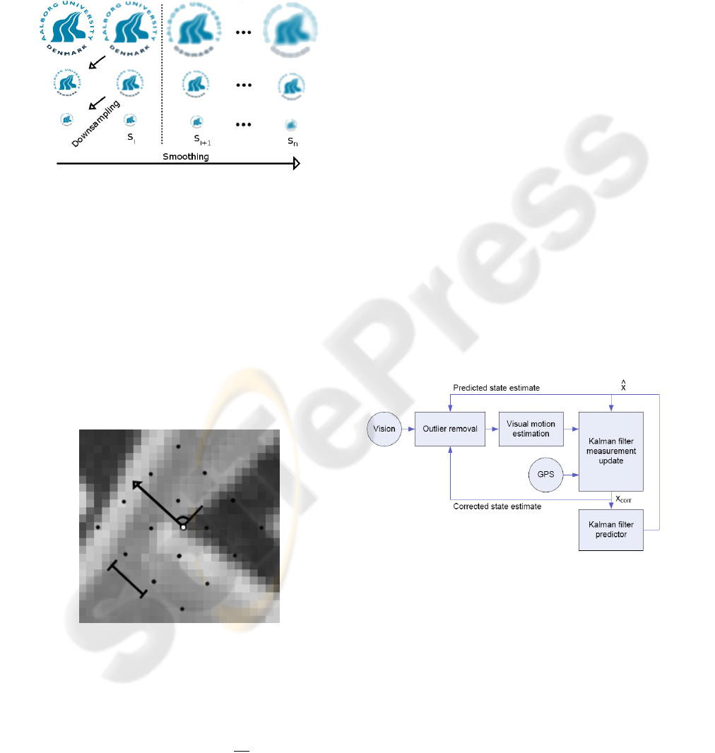
2.1.3 Feature Detection, Description, and
Matching
For feature detection, description and matching the
method introduced by (Brown et al., 2005) with mi-
nor modifications is used. First the input image is in-
crementally smoothed with an Gaussian kernel. Next
an image pyramid is constructed by down sampling
of the image at the scale just above the current, as il-
lustrated in Figure 1. Extreme locations is found by
Harris-Corner detection in the image smoothed with
a variance s
i
larger than one by the Harmonic mean
method with a threshold of 10. The extreme points
are hereafter denoted as landmarks. Finally, the sub
pixel precision of the landmarks are found by a Taylor
expansion (up to the quadric term) at the landmarks
(Brown and Lowe, 2002).
Figure 1: Illustration of the scale-space approach.
The landmarks are described by their orientation
in a window of size 28x28 (corresponding to a Gaus-
sian kernel with σ = 4.5) and sampling of grey level
values in their 40x40 neighborhood in the scale above
the current, i.e. s
i+1
where s
i
is the variance at the
current scale. The grey level values are sampled in
a grid with a spacing of 5 pixels rotated according to
the landmarks orientation. To adjust for sub pixel pre-
cision bilinear interpolation is used around the sam-
pling location to estimate the grey level values, as il-
lustrated in Figure 2. This gives a feature vector for
each landmark consisting of 8x8 grey level values.
Figure 2: Illustration of the landmarks orientation and grid
for sampling of grey values. For clarity only a 4x4 grid is
illustrated.
Before matching the feature vector is standardized
by substraction the mean and dividing by its standard
deviation. Matching is done along the epipolar lines
using the similarity measure sim =
1nn
2nn
, i.e. the ratio
of the best and second best match. For selection of
candidates only sim with a values less than 0.5 is used
for matching between successive stereo image pairs.
For candidates with successful matching a mean fea-
ture vector is determined as the average between the
two vectors from each of the stereo images.
Matching between successive stereo image pairs
is achieved by using the average feature vector with
the same similarity measure and threshold. Success-
fully matched landmarks are reconstructed and pro-
jected onto the ground plane to give Q
c
and Q
p
.
2.2 Data Fusion
The visual motion and GPS position estimates is
fused by a Kalman filter (KF). Let χ = (x
w
,y
w
,v
x
,v
y
)
be the state vector in the KF where (x
w
,y
w
) is the posi-
tion in the global coordinate system and (v
x
,v
y
) is the
velocity of the robot. The assumed dynamic model
assumes a constant velocity and is given by
χ(k+ 1) =
1 0 1 0
0 1 0 1
0 0 1 0
0 0 0 1
χ(k+ 1) + Σ
p
(5)
where the process noise Σ
p
∈ NID(0,0.01· I) is nor-
mally independent distributed with a covariance cor-
responding to 10 cm. The filter is updated with mea-
surements from the vision and GPS sensors as out-
lined in Figure 3.
Figure 3: Kalman filter setup. Errors in the image point sets
are detecting and discarding using KF estimates.
Since the KF tracks the state estimate over time,
it is possible to use the prior estimate of the state to
rejects outliers in the image points by comparing the
magnitude of the predicted movement of the KF to the
movement between the corresponding points in point
sets Q
c
and Q
p
.
The magnitude of the movement η between the
corrected χ
corr
and the predicted
ˆ
χ position of the KF
is:

η =
q
(χ
corr
−
ˆ
χ)
T
(χ
corr
−
ˆ
χ) (6)
η is used to select plausible corresponding points in
Q
c
and Q
p
according to:
ηα < δ < ηβ (7)
where δ is the distance between two point pairs in
Q
c
and Q
p
, i. e. δ =
p
(c
i
− p
i
)
T
(c
i
− p
i
). α and
β are constants set to respectively 0.5 and 2. Visual
motion estimation was only considered robust when
more than 15 point pairs had a δ value within the lim-
its according to eq. 7.
2.2.1 Data Alignment
Angular alignment of the local robot (stereo) coordi-
nate system and the global GPS coordinate system is
achieved using an estimate of the orientation θ. This
estimate is generally available directly from the vi-
sual motion estimates, see eq. 2. The experimental
setup, however, provoke the vision system into situa-
tions where no valid vision data is available, and an
alternative source of angular alignment data is hence
required. Such information may be obtained from a
magnetometer, by additional modeling and inclusion
in the filter model, or by using an attitude type GPS
receiver. In the current study, the rotation estimates
were obtained from the TANS vector GPS (see sec-
tion 2.3) in cases where θ is not available from the vi-
sion sensor. Consequently, every time the visual mo-
tion estimation becomes valid after a period of invalid
data, it begins at the correct angle and from here er-
rors accumulate until it is regarded as being invalid
again.
2.3 Experimental Setup
To obtain ground truth as correct as possible a cali-
brated stereo camera setup with the specifications ac-
cording to table 1, was mounted on a iron pivot with
a diameter of 21.78 meters, see Figure 4.
Table 1: Specifications of the stereo setup.
Parameter Value
Baseline, T 60 cm
Height 75 cm
Focal length, f 8 mm
F-value 1.4
Camera tilt angle 45
◦
Image resolution 640 × 512
Pixel size, △ x 6.0 x 6.0 µ m
Left Camera
Right Camera
RTK GPS
TANS Vector
Pivot
Pivot radius (r)
Driving direction
Figure 4: Illustration of the experimental setup.
At the center of the stereo vision setup a Top-
Con RTK GPS-module was placed. At approximately
17 meter from the center a Trimble Advanced Nav-
igation System (TANS), vector GPS attitude mea-
surement system was placed. The TANS vector is
a four-antenna, six-channel Global Positioning Sys-
tem (GPS) receiver system which provides standard
or differentially corrected (DGPS) position, velocity,
time, and 3-dimensional attitude (azimuth, pitch, and
roll) to external data terminals. Corresponding read-
ings from the GPS module, the TANS vector and the
stereo setup was recorded. The TANS vector is re-
garded as ground truth and operates with an accuracy
of 0.5
◦
(RMS). The pivot is drawn smoothly back-
wards clockwise with an angular velocity of approx-
imately 0.7
rad
s
. The ground surface at the setup has
only minor undulations and may be regarded as pla-
nar.
The landscape surrounding the pivot is open field.
At the end of the circular movement of the pivot a
tractor with a trailer and a Van was placed closed to
the circumference to simulate the situation that the
GPS gets occluded and the vision system gets reliable
landmarks, see Figure 5.
Reliable covariance estimates are not directly
available from the TopCon RTK GPS-module. In-
stead an estimate was formed by taking five GPS read-
ings on either side of the current position. The sum of
squares and cross product matrix of the error between
the position of the TANS vector readings and the GPS
for the 11 samples was used as an estimate of the co-
variance of the GPS.
3 RESULTS
In Figure 6 the percentage variance explained by the
first eigenvalue of the covariance matrices for respec-
tively Q
c
and Q
p
is plotted. Except at the beginning
and at the end of the experiment the first eigenvalue
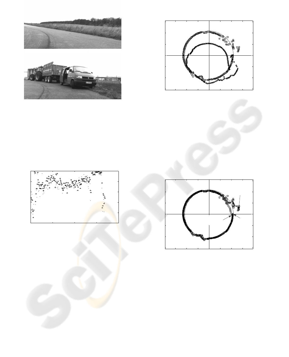
Figure 5: Images from the beginning and end of the image
series.
account for about 90% of the variance in the point
sets. At the end of the series the point sets is not as
dominantly distributed in one dimension which is in
good agreement with what is to be expected from the
experimental setup.
0 50 100 150 200
50
60
70
80
90
100
Image number
Percent explained variance
Figure 6: Percentage explained variance by the first eigen-
value of the covariance matrix. Dot, the current point set,
Q
c
. Cross the previous point set, Q
p
.
The ”raw” measurements from the experiment are
illustrated in Figure 7. The raw angular readings from
the TANS measurements are multiplied by the radius
(21.78 meters) i.e. the distance from the center of
pivot and to the center of the Topcon GPS module.
In this way the ground truth for the experiment is ob-
tained.
The visual estimates are given in a local robot co-
ordinate system. The local estimates are projected
onto the global GPS defined coordinate system using
the cumulative value of θ. From the figure it is obvi-
ous that the visual motion estimates are most reliable
at the end of the series. In contrast the GPS record-
ings are stable until the end of the trajectory where it
gets occluded by the obstacles placed along the cir-
cumference.
−30 −20 −10 0 10 20 30
−30
−20
−10
0
10
20
30
Meter
Meter
Figure 7: Raw measurements. Dot, readings from the
TANS setup. Box, GPS readings. Star, accumulated move-
ment by the visual motion estimation.
In Figure 8 the Kalman filtered position estimates
with and without the visual motion estimates is plot-
ted. From the figure it obvious that inclusion of
the visual motion estimate makes the position more
smooth, especially at the end of the experiment.
−30 −20 −10 0 10 20 30
−30
−20
−10
0
10
20
30
Meter
Meter
End, KF only
with GPS
End, KF with GPS
and Visual Motion
Start
Figure 8: Kalman filtered data for the experiment. Dot,
readings from the Tans setup. Box, GPS readings. Cross,
KF position estimates using only GPS readings as input.
Circle, KF position estimates including the visual motion
estimates.
Table 2 and Figure 9 summaries and illustrate how
the position estimates from the Kalman filter with
and without visual motion estimation deviate from the
ground truth. From the table it may be noticed that
for the mean deviation there is no difference for the
two approaches. However, for the standard, maxi-
mum, and deviation from ”closing the circle” there
are significant smaller deviation for the Kalman filter
supported by visual motion estimation.
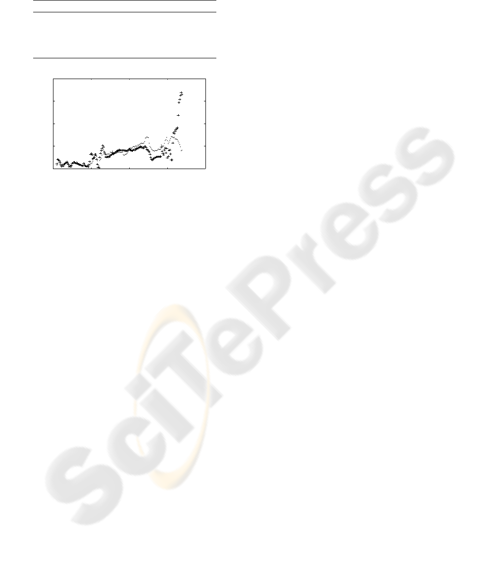
Table 2: Deviation from the ground truth of the position es-
timates given by the Kalman filter. GPS, only GPS readings
included in the KF. Visual motion, GPS readings and visual
motion estimates included in the KF.
Deviation (meters) GPS Visual motion
Mean 1.38 1.39
Std 1.16 0.80
Max 6.76 2.83
Closing the circle 6.58 1.63
0 50 100 150 200
0
2
4
6
8
Image number
Deviation in meter
Figure 9: Deviation of the Kalman filtered position estimate
relative to the position from the TANS vector. Cross, only
GPS. Dot, visual motion estimation included in the KF.
4 DISCUSSION
In this study the problem of using visual motion es-
timation to support GPS localization under non ideal
condition for either technologies. A significant effort
has been put into establishing ground truth estimate of
the position a prerequisite for evaluation of the prob-
lem addressed.
The α and β has in this study been set to constant
values. In a more dedicated filter the two constant
should be connected to the covariance structure of the
corrected and predicted state estimate of the KF.
The visual motion estimation has to some de-
gree been put into a favorable situation by letting the
method start at the right rotation angle for alignment
after a drop-out. Whether other sensor modalities or
landmarks can provide the ”correct” angle at a given
position has not been addressed. But what its demon-
strated is that the introduced simple visual motion
method together with the KF outlier detection is able
to enhance the localization estimate where the GPS
is occluded without degrading the estimate where the
visual estimate is unreliable.
5 CONCLUSION
We presented a system for motion estimation of
robots or vehicles operating in an outdoor environ-
ment. The outdoor open field application presents
some specific problems, such as GPS signal occlu-
sion, and visual landmarks that are primarily dis-
tributed in the horizon on a line. We benefited from
the complimentary strengths of vision and GPS, by
fusing the motion estimates in a Kalman filter while
using the filter estimates to remove outliers in the vi-
sual landmark matching. Assuming vehicle motion
on a plane, and focusing on a dimensional image point
distribution, allowed visual motion estimation based
on analysis of the image point set covariance struc-
ture. The system was tested under realistic open field
outdoor conditions. The system was tested against
ground truth and the fusion of GPS and vision proved
to significantly reduce the variance compared to a sit-
uation with only GPS.
ACKNOWLEDGEMENTS
This work is part of the project Across under the Na-
tional Research programme Sustainable Technology
in Agriculture.
REFERENCES
Brown, M. and Lowe, D. (2002). Invariant features from in-
terest point groups. In Proceedings of the 13th British
Machine Vision Conference, pages 253–262, Cardiff.
Brown, M., Szeliski, R., and Winder, S. (2005). Multi-
image matching using multi-scale oriented patches. In
CVPR05, pages 510–517, San Diego.
Jackson, J. E. (1991). A user’s guide to principal compo-
nents. John Wiley & Sons Inc.
Matthies, L. (1989). Dynamic Stereo Vision. PhD thesis,
Carnigie-Mellon University.
Matthies, L. and Shafer, S. (1987). Error modeling in
stereo navigation. Journal of Robotics and Automa-
tion, 3(3):239–248.
Nister, D. (2003). Preemptive ransac for live structure and
motion estimation. In IEEE International Conference
on Computer Vision, pages 199–206.
Nister, D., Naroditsky, O., and Bergen, J. (2006). Visual
odometry for ground vehicle applications. Journal of
Field Robotics, 23:3–20.
Olson, C. F., Matthies, L. H., Schoppers, M., and Mai-
moneb, M. W. (2003). Rover navigation using stereo
ego-motion. Robotics and Autonomous Systems,
43:215229.
Stephen Se, Lowe, D. G. and Little, J. (2005). Vision based
global localization and mapping for mobile robots.
IEEE Transactions on Robotics, 21(3):364–375.
