
VIDEO MODELING USING 3-D HIDDEN MARKOV MODEL
Joakim Jitén and Bernard Merialdo
Institute Eurecom, BP 193, 06904 Sophia-Antipolis, France
Keywords: Hidden Markov Model, three-dimensional HMM, video modeling, object tracking.
Abstract: Statistical modeling methods have become critical for many image processing problems, such as
segmentation, compression and classification. In this paper we are proposing and experimenting a
computationally efficient simplification of 3-Dimensional Hidden Markov Models. Our proposed model
relaxes the dependencies between neighboring state nodes to a random uni-directional dependency by
introducing a three dimensional dependency tree (3D-DT HMM). To demonstrate the potential of the model
we apply it to the problem of tracking objects in a video sequence. We explore various issues about the
effect of the random tree and smoothing techniques. Experiments demonstrate the potential of the model as
a tool for tracking video objects with an efficient computational cost.
1 INTRODUCTION
A number of researches have introduced systems
that employ statistical modeling techniques to
segment, classify, and index images (Lefevre 2003,
Kato 2004, Joshi 2006). Recent years have seen
substantial interest and activity devoted to the
exploration of various hidden Markov models for
image and video applications, which have earlier
become a key technology for many applications such
as speech recognition (Rabiner 1983) and language
modeling.
The success of HMMs is largely due to the
discovery of an efficient training algorithm, the
Baum-Welch algorithm (Baum 1966), which allows
estimating the numerical values of the model
parameters from training data. Given the impressive
success of HMMs for solving 1-Dimensional
problems, it appears natural to extend them to multi-
dimensional problems, such as image and video
modeling. However, the challenge is that the
complexity of the algorithms grows tremendously in
higher dimensions, so that, even in two dimensions,
the usage of full HMM often becomes prohibitive in
practice (Levin 1992), at least for realistic problems.
Many simplification approaches have been proposed
to overcome this complexity of 2D-HMMs (Joshi
2006, Mohamed 2000, Perronnin 2003, Brand 1997,
Fine 1998). The main disadvantage of these
approaches is that they only provide approximate
computations, so that the probabilistic model is no
longer theoretically sound or greatly reduce the
vertical dependencies between states, as it is only
achieved through a single super-state. For three
dimensional problems, HMMs have been very rarely
used, and only on simplistic artificial problems
(Joshi 2006).
In this paper we propose an efficient type of
multi-dimensional Hidden Markov Model; the
Dependency-Tree Hidden Markov Model
(DT HMM) (Merialdo 2005) which is theoretically
sound while preserving a modest computational
feasibility in multiple dimensions (Jiten 2006). In
section two, we recall our proposed model for two
dimensions, then we show how it is easily extended
to three dimensions. Then, in section three, we
experiment this model on the problem of tracking
objects in a video. We explain the initialization and
the training of the model, and illustrate the tracking
with examples of a real video.
2 DEPENDENCY-TREE HMM
In this section, we briefly recall the basics of
2D-HMMs and describe our proposed DT HMM
(Merialdo 2005).
191
Jitén J. and Merialdo B. (2007).
VIDEO MODELING USING 3-D HIDDEN MARKOV MODEL.
In Proceedings of the Second International Conference on Computer Vision Theory and Applications - IFP/IA, pages 191-198
Copyright
c
SciTePress
2.1 2D-HMM
The reader is expected to be familiar with
1-D HMM. We denote by O={o
ij
, i=1,…m,
j=1,…,n} the observation, for example each o
ij
may
be the feature vector of a block (i,j) in the image. We
denote by S = {s
ij
, i=1,…m, j=1,…,n} the state
assignment of the HMM, where the HMM is
assumed to be in state s
ij
at position (i,j) and produce
the observation vector o
ij
. If we denote by λ the
parameters of the HMM, then, under the Markov
assumptions, the joint likelihood of O and S given λ
can be computed as:
()()
λλ
λλλ
,,,
)(),(),(
1,,1 −−
∏
=
=
jijiij
ij
ijij
ssspsop
SPSOPSOP
(1)
If the set of states of the HMM is {s
1
, … s
N
},
then the parameters λ are:
• the output probability distributions p(o | s
i
)
• the transition probability distributions p(s
i
| s
j
,s
k
).
Depending on the type of output (discrete or
continuous) the output probability distribution are
discrete or continuous (typically a mixture of
Gaussian distribution).
2.2 2D-DT HMM
The problem with 2-D HMM is the double
dependency of s
i,j
on its two neighbors, s
i-1,j
and s
i,j-1
,
which does not allow the factorization of
computation as in 1-D, and makes the computations
practically intractable.
(i-1,j)
(i,j-1) (i,j)
Figure 1: 2-D Neighbors.
Our idea is to assume that s
i,j
depends on one
neighbor at a time only. But this neighbor may be
the horizontal or the vertical one, depending on a
random variable t(i,j). More precisely, t(i,j) is a
random variable with two possible values :
⎩
⎨
⎧
−
−
=
5.0)1,(
5.0),1(
),(
probwithji
probwithji
jit
(2)
For the position on the first row or the first
column, t(i,j) has only one value, the one which
leads to a valid position inside the domain. t(0,0) is
not defined. So, our model assumes the following
simplification:
⎪
⎩
⎪
⎨
⎧
−=
−=
=
−
−
−−
)1,(),()(
),1(),()(
),,(
1,,
,1,
1,,1,
jijitifssp
jijitifssp
tsssp
jijiH
jijiV
jijiji
(3)
If we further define a “direction” function:
⎩
⎨
⎧
−=
−=
=
)1,(
),1(
)(
jitifH
jitifV
tD
(4)
then we have the simpler formulation:
)(),,(
),(,)),((1,,1, jitjijitDjijiji
ssptsssp =
−−
(5)
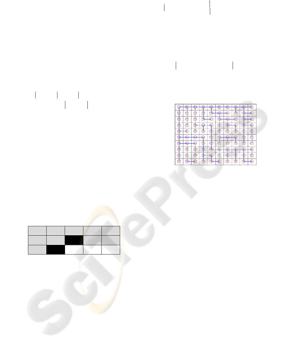
Note that the vector t of the values t(i,j) for all
(i,j) defines a tree structure over all positions, with
(0,0) as the root. Figure 2 shows an example of
random Dependency Tree.
Figure 2: Example of a Random Dependency Tree.
The DT HMM replaces the N
3
transition
probabilities of the complete 2-D HMM by 2N
2
transition probabilities. Therefore it is efficient in
terms of storage and computation. Position (0, 0) has
no ancestor. We assume for simplicity that the
model starts with a predefined initial state s
I
in
position (0, 0). It is straightforward to extend the
algorithms to the case where the model starts with an
initial probability distribution over all states.
2.3 3-D DT HMM
The DT HMM formalism is open to a great variety
of extensions and tracks; for example other ancestor
functions or multiple dimensions. Here we consider
the extension of the framework to three dimensions.
We consider the case of video data, where the two
dimensions are spatial, while the third dimension is
temporal. However, the model could be applied to
other interpretations of the dimensions as well.
In three dimensions, the state s
i,j,k
of the model
will depend on its three neighbors s
i-1,j,k
, s
i,j-1,k
, s
i,j,k-1
.
This triple dependency increases the number of
transition probabilities in the model, and the
computational complexity of the algorithms such as
Viterbi or Baum-Welch. However the use of a 3-D
Dependency Tree allows us to estimate the model
VISAPP 2007 - International Conference on Computer Vision Theory and Applications
192
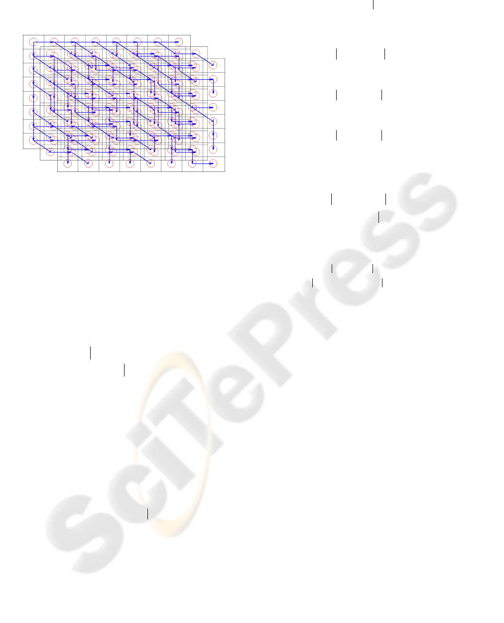
parameters along a 3-D path (see Figure 3) which
maintains a linear computational complexity.
Figure 3: Random 3-D Dependency Tree.
The “direction” function for the 3-D tree becomes:
⎪
⎩
⎪
⎨
⎧
−=
−=
−=
=
)1,,(
),1,(
),,1(
)(
kjitifZ
kjitifH
kjitifV
tD
(6)
In 3-D modeling, let us denote the observation
vector o
ijk
as the observation of a block (i,j,k) in a
sequence of 2-D images. In an analogous way the
HMM state variables s
ijk
represents the state at
position (i,j,k) that produce the observation vector
o
ijk
. Thus now we can extend (5) to three
dimensions:
)(
),,(
),,(,,)),,((
1,,,1,,,1,,
kjitkjikjitD
kjikjikjikji
ssp
tssssp
=
−−−
(7)
In this paper we use Viterbi training to fit our
model, thus we need to iterate the search for the
optimal combination of states and then re-estimate
the model parameters.
2.3.1 3-D Viterbi Algorithm
The Viterbi algorithm finds the most probable
sequence of states which generates a given
observation O:
),(Argmax S
^
tSOP
S
=
(8)
Let us define T(i,j,k) as the sub-tree with root (i,j,k),
and define β
i,j,k
(s) as the maximum probability that
the part of the observation covered by T(i,j,k) is
generated starting from state s in position (i,j). We
can compute the values of β
i,j,k
(s) recursively by
enumerating the positions in the opposite of the
raster order, in a backward manner:
• if (i,j,k) is a leaf in T(i,j,k):
)()(
,,,,
sops
kjikji
=
β
(9)
• if (i,j,k) has only an horizontal successor, by
adopting equation (7) we get:
)'()'(max)()(
,1,
'
,,,,
ssspsops
kjiH
s
kjikji +
=
ββ
(10)
• if (i,j,k) has only a vertical successor:
)'()'(max)()(
,,1
'
,,,,
ssspsops
kjiV
s
kjikji +
=
ββ
(11)
• if (i,j,k) has only a z-axis successor:
)'()'(max)()(
1,,
'
,,,,
ssspsops
kjiZ
s
kjikji +
=
ββ
(12)
• if (i,j,k) has both an horizontal and a vertical
successors (and respectively for the other two
possible combinations):
(
)
()
)'()'(max
)'()'(max)()(
,,1
'
,1,
'
,,,,
sssp
ssspsops
kjiV
s
kjiH
s
kjikji
+
+
=
β
ββ
(13)
• if (i,j,k) has both an horizontal, a vertical and z-
axis successors:
(
)
(
)
(
)
)'()'(max)'()'(max
)'()'(max)()(
1,,
'
,,1
'
,1,
'
,,,,
ssspsssp
ssspsops
kjiZ
s
kjiV
s
kjiH
s
kjikji
++
+
=
ββ
ββ
(14)
Then the probability of the best state sequence
for the whole image is β
0,0,0
(s
I
). Note that this value
may also serve as an approximation for the
probability that the observation was produced by the
model.
The best state labeling is obtained by assigning
s
0,0,0
= S
I
and selecting recursively the neighbor
states which accomplish the maxima in the previous
formulas.
Note that the computational complexity of this
algorithm remains low: we explore each block of the
data only once, for each block we only have to
consider all possible states of the model, and for
each state, we have to consider at most three
successors. Therefore, if the video data is of size (W,
H, T), and the number of states in the model is S, the
complexity of the Viterbi algorithm for 3D-DT
HMMs is only O(WHTS).
2.3.2 Relative Frequency Estimation
The result of the Viterbi algorithm is a labeled
observation, i.e. a sequence of images where each
output block has been assigned a state of the model.
Then, it is straightforward to estimate the transition
probabilities by their relative frequency of
occurrence in the labeled observation, for example:
VIDEO MODELING USING 3-D HIDDEN MARKOV MODEL
193

)(
)',(
),'(
,
sN
ssN
tssp
tH
H
=
(15)
where
)',(
,
ssN
tH
is the number of times that
state s’ appears as a right horizontal neighbor of
state s in the dependency tree t, and
)(sN the
number of times that state s appears in the labeling .
(This probability may be smoothed, for example
using Lagrange smoothing). The output probabilities
may be also estimated by relative frequency in the
case of discrete output probabilities, or using
standard Multi-Gaussian estimation in the case of
continuous output probabilities.
With these algorithms we can estimate the model
parameters from a set of training data, by so called
Viterbi training: starting with an initial labeling of
the observation (either manual, regular or random),
or an initial model, we iteratively alternate the
Viterbi algorithm to generate a new labeled
observation and Relative Frequency estimation to
generate a new model. Although there is no
theoretical proof that this training will lead to an
optimal model, this procedure is often used for
HMMs and has proven to lead to reasonable results.
Note that with 3D-DT HMMs, the Baum-Welch
algorithm and the EM reestimation lead to a
computational complexity that is similar to the
Viterbi algorithm, so that a true Maximum
Likelihood training is computationally feasible in
this case. We have not yet implemented those
algorithms, but started with the simple Viterbi and
Relative Frequency for our initial experimentations
on 3D video data.
3 EXPERIMENTS
Video can be regarded as images indexed with time.
Considering the continuity of consecutive frames, it
is often reasonable to assume local dependencies
between pixels among frames. If a position is (i,j,t),
it could depend on the neighbors (i-1,j,t), (i,j-1,t),
(i,j,t-1) or more. Our motivation is to model these
dependencies by a 3-D HMM. As described in 2.3,
images are represented by feature vectors on an
array of 2-D images.
To investigate the impact of the time-dimension
dependency we explore the ability of the model to
track objects that cross each other or pass behind
another static object. To this end we have chosen a
video sequence with two skiers that pass behind
each other and static markers that remain fixed on
the scene. The video contains 24 frames.
The method is mainly composed of two phases:
the training phase and the segmentation phase. In the
training phase, the process learns the unknown
HMM parameters using the Viterbi training
explained in section 2. In the segmentation phase,
the process performs a spatio-temporal segmentation
by performing a 3-D Viterbi state alignment.
3.1 Model Training
We consider a 3-D DT HMM with 9 states and
continuous output probabilities. Our example video
contains 24 frames which are divided into 44 x 30
blocks; hence the state-volume has dimension
44 x 30 x 24. For each block, we compute a feature
vector as the average and variance of the CIE LUV
color space coding {L
μ
,U
μ
,V
μ
, L
σ
,U
σ
,V
σ
} combined
with six quantified DCT coefficients (Discrete
Cosine Transform). This constitutes the observation
vector o
ijk
.
The choice of the observation vector is motivated
by the fact that we use GMMs, it was desirable to
use features which are Gaussian distributed and are
as much uncorrelated as possible. Further as it is
well known that histogram output as features has
highly skewed probability distributions, we decided
to use means and variances for color descriptors.
DCT coefficients were chosen for their
discriminative ability of energies in the frequency
domain. The LUV color coding is often preferred for
its good perception correlation properties.
Initial Model
The first step of the training is to build the initial
model. To build initial estimates of the output
probabilities, we manually annotated regions in the
first two frames of the video by segmenting the
image into arbitrary shaped regions using the
algorithm proposed in (Felzenszwalb 2006) and then
manually associating each region with a class
category. As it can be seen in the figure below, the
segmentation is rather coarse, which means that
parts of the background may be included in the
object regions.
Figure 4: Training image and initial state configuration
using annotated regions.
VISAPP 2007 - International Conference on Computer Vision Theory and Applications
194
The image was labeled using four different
categories: background, skier1, skier2 and marker
(static object in the scene). Since semantic video
regions do not usually have invariant visual
properties, we assign a range of states to allow for a
flexible representation for each category (or sub-
class). The sub-class background can for instance
have the colors: white or light grey with different
texture properties such as regular or grainy. The
table below lists the sub-classes and their associated
number of states.
Table 1: Number of states for each sub-class.
Sub Class No. states
Background 3
Skier 1 2
Skier 2 2
Marker 2
4 sub-classes 9 states
Each state has an output distribution which is
represented by a GMM (Gaussian Mixture Model)
with five components. To estimate these
probabilities, we collect the observation vectors for
each category, cluster them into the corresponding
number of states, and perform a GMM estimation on
each cluster.
The transition probabilities are estimated by
Relative Frequency on the first frame for the spatial
dependencies, and by uniform distribution for the
temporal dependency.
3D Dependency Tree
The observation volume has size 44 x 30 x 24, and
each observation is supposed to be generated by a
hidden state. We build a random 3D dependency tree
(see Figure 3) by creating one node for each
observation, and randomly selecting an ancestor for
each node out of the three possible directions:
horizontal, vertical and temporal. The border nodes
have only two (if they lie on a face of the volume),
one (if they lie on an edge) or zero (for the root
node) possible ancestors.
In our experiments, we generated a random 44 x
30 x 24 dependency tree which contains:
Table 2: Number of ancestors for each direction.
Direction No. ancestors
horizontal 10 604
vertical 10 694
temporal 10 382
Total 31 680
Training
As previously explained, we perform Viterbi
training by iteratively creating a new labeling over
the observations, using Viterbi training, and
generating a new model, using Relative Frequency
estimation. The iterations stop when the increase in
the observation probability p(O | S, t) is less than a
threshold.
Data Size vs. Model Complexity
According to the Bayesian information criterion
(BIC) the quality of the model is proportional to the
logarithm of the number of training samples and the
complexity of the model [M. Nishida]. Thus since
our training data is sparse, we shall use a small
mixture size. The necessary complexity of the GMM
depends of the data class to model, which in this
case is relatively uniform since the image is
segmented into annotated object regions (each
represented by a number of states as shown in
Table 1).
The EM-algorithm is used for training, which has
a tendency to make very narrow Gaussians around
sparse data points. To avoid this potential problem
we construct the GMMs so that there are always a
smallest number of samples in each component, and
we constrain the variance to a minimum threshold.
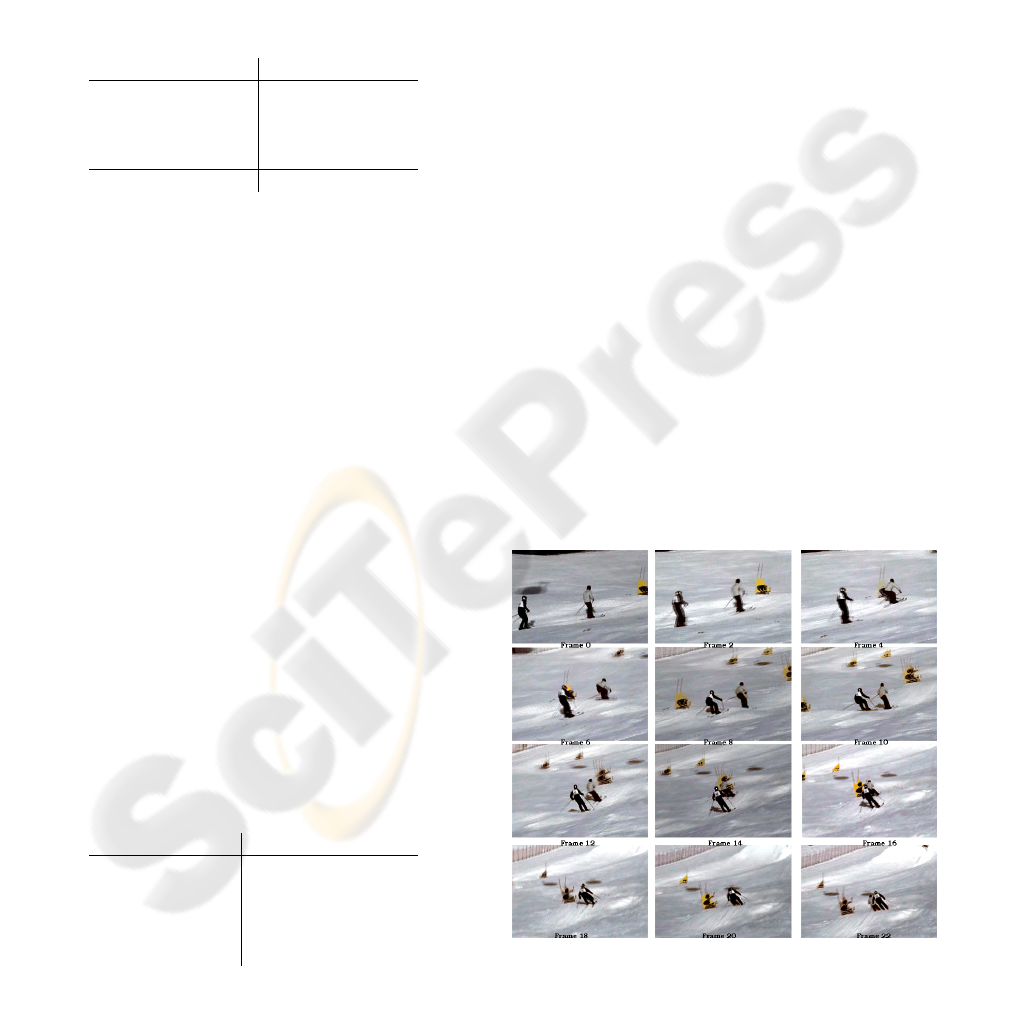
3.2 Object Tracking
The original video contains two skiers passing
yellow markers on a snowy background with
shadows. Figure 5 depicts every second frame of the
sequence.
Figure 5: Original video sequence; first frame in upper left
corner, followed by every second frame.
VIDEO MODELING USING 3-D HIDDEN MARKOV MODEL
195
The first frame was manually annotated and used
to estimate the initial model, while the following
frames constitute the 3D observation on which the
Viterbi training was performed. Then, we use the
trained model to get a final labeling of the complete
3D observation. In the final labeling, each
observation block is assigned to a single state of the
model. The final labeling provides a spatio-temporal
segmentation of the 3D observation. As the states of
the model correspond to semantic categories, it is
possible to interpret the content of specific blocks in
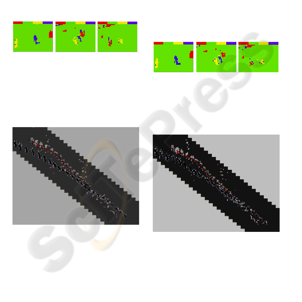
the video sequence. Figure 6 shows the segment
classification for frame 1, 12 and 24.
Figure 6: Frame segmentation in the final labeling (a)
frame 1, (b) frame 12, (c) frame 24.
Object tracking is then performed easily, by
selecting in each frame the blocks which are labeled
with the corresponding semantic category. For
example, we can easily create a video sequence
containing only the skiers by switching off the states
for the background- and marker-classes as shown in
Figure 7.
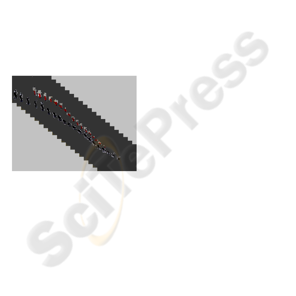
Figure 7: Object tracking of two skiers.
We can see in the figure above that some blocks
are incorrectly assigned to the skier categories. An
explanation for this fact maybe that with a single
dependency tree, many blocks inside the video
correspond to leaves in the tree, and therefore are
not constrained by any successor. This motivates the
combination of several dependency trees so that no
node is left without any constraints from its
successors.
Complementary Dual Trees
We would like to consider dependencies in every
direction for each node. Therefore, given a random
dependency tree t, it is reasonable to consider its
dual trees, which are trees where for each node, we
select one direction among those not used in t
(except when the node has a single possible
ancestor). Note that in 2D, the dual tree is unique,
while in 3D, there are a lot of different dual trees for
a given t. However, we can select a pair of
complimentary dual trees so that every possible
dependency for every node appears at least once in
one of the three trees. We use a majority vote to
compute the best labeling for the triplet of trees.
Figure 8 show the result of the segmentation on
various frames.
Figure 8: Frame segmentation using complementary dual
trees, (a) frame 1, (b) frame 12, (c) frame 24
.
As previously, we can construct a video
sequence showing only the tracked objects,.
Unfortunately, this combination shows only minor
improvement over the segmentation with a single
tree.
Figure 9: Perspective view of object tracking using
complementary dual trees.
Multiple tree labeling
Although using a triplet of tree and complimentary
dual trees takes every dependency from every node
into account, this is only a local constraint between
neighbors, which may not be sufficient to propagate
the constraint to a larger distance. Notice that, for
every pair of nodes (not necessarily neighbors),
VISAPP 2007 - International Conference on Computer Vision Theory and Applications
196
there is always a dependency tree where one of the
nodes will be the ancestor of the other. So, the idea
now is to use a large number of trees (ideally all, but
they are too numerous), so that we increase the
chance of long-distance dependency between non-
neighbor nodes.
For each dependency tree, we can compute the
best state alignment, then use a majority vote to
select the most probable state for each block. This is
an approximation for the probability of being in this
state for this block during the generation of the
observation with an unknown random tree (a better
estimate could be obtained using the extended
Baum-Welch algorithm, but we have not
implemented this algorithm yet, so we just use the
Viterbi algorithm here). Figure 10 shows the video
obtained with this multiple tree labeling, using a set
of 50 randomly generated trees. As can be seen from
these results, the objects are much clearly defined in
this experiment, and most of the noise in the labeling
has disappeared.
Figure 10: Object tracking with smoothing over 50
random trees.
4 CONCLUSION
In this paper, we have proposed a new
approximation of multi-dimensional Hidden Markov
Model based on the idea of Dependency Tree. We
have focused on the definition and use of 3D
HMMs, a domain which has been very weakly
studied up to now, because of the exponential
growth of the required computations.
Our approximation leads to reasonable
computation complexity (linear with every
dimension). We have illustrated our approach on the
problem of video segmentation and tracking. We
have detailed the application of our model on a
concrete example. We have also shown that some
artifacts due to our simplifications can be greatly
reduced by the use of a larger number of dependency
trees.
In the future, we plan to explore other
possibilities of 3D HMMs, such as classification,
modeling, etc… on various types of video. Because
of the learning capabilities of HMMs, we believe
that this type of model may find a great range of
applications.
REFERENCES
A. Baumberg and D. Hogg. Learning flexible models
from image sequences. In ECCV, volume 1, pages
299-308, Stockholm, Sweden, May 1994.
N. Paragios and R. Deriche. A PDE-based Level Set
Approach for Detection and Tracking of Moving
Objects. Technical Report 3173, INRIA, France, May
1997.
D. Koller, J. W. Weber, and J. Malik, Robust multiple car
tracking with occlusion reasoning, in European
Conference on Computer Vision, pp. 189--196, LNCS
800, springer-Verlag, May 1994.
S. Lefevre, E. Bouton, T. Brouard, N. Vincent, "A new
way to use hidden Markov models for object tracking
in video sequences", IEEE International Conference
on Image Processing (ICIP), Volume 3, page 117-120
- September 2003.
Kato, J. Watanabe, T., Joga, S., Liu, Y., Hase, H., An
HMM/MRF-based stochastic framework for robust
vehicle tracking, ITS(5), No. 3, September 2004, pp.
142-154. IEEE Abstract. IEEE Top Reference. 0501.
Perronnin, F.; Dugelay, J.-L.; Rose, K., “Deformable face
mapping for person identification”, International
Conference on Image Processing, Volume 1, 14-17
Sept. 2003 Page(s):I - 661-4.
Joshi, D. Jia Li Wang, J.Z., A computationally efficient
approach to the estimation of two- and three-
dimensional hidden Markov models, Image
Processing, IEEE Transactions on, July 2006.
L.R. Rabiner. "A tutorial on HMM and selected
applications in speech recognition". In Proc. IEEE,
Vol. 77, No. 2, pp. 257-286, Feb. 1989.
LE. Baum and T. Petrie, Statistical Inference for
Probabilistic Functions of Finite State Markov Chains,
Annual Math., Stat., 1966, Vol.37, pp. 1554-1563.
Levin, E.; Pieraccini, R.; Dynamic planar warping for
optical character recognition, IEEE International
Conference on Acoustics, Speech, and Signal
Processing, , Volume 3, 23-26 March 1992
Page(s):149 – 152.
Mohamed, M. A., Gader P.: Generalized Hidden Markov
Models-Part I: Theoretical Frame-works, IEEE
Transaction on Fuzzy Systems, February, 2000, Vol.8,
No.1, pp. 67-81
M. Nishida and T. Kawahara, “Unsupervised Speaker
Indexing Using Speaker Model Selection based on
VIDEO MODELING USING 3-D HIDDEN MARKOV MODEL
197

Bayesian Information Criterion,” Proc. ICASSP, Vol.
1, pp. 172-175, 2003.
Brand, M., Oliver, N. and Pentland, A.: Coupled hidden
Markov models for complex action recognition. In
Proceedings, CVPR, pages 994--999. IEEE Press,
1997
Fine S., Singer Y., Tishby, N.: The hierarchical hidden
Markov model: Analysis and applications," Machine
Learning 32(1998)
Merialdo, B; Dependency Tree Hidden Markov Models,
Research Report RR-05-128, Institut Eurecom, Jan
2005
J. Jiten, B. Merialdo, "Probabilistic Image Modeling With
Dependency-Tree Hidden Markov Models", WIAMIS
- International Workshop on Image Analysis for
Multimedia Interactive Services, Korea 2006.
P. F. Felzenszwalb , D. P. Huttenlocher, Image
Segmentation Using Local Variation, Proc. of the
IEEE Computer Society Conference on Computer
Vision and Pattern Recognition, p.98-vices, Korea
2006.
VISAPP 2007 - International Conference on Computer Vision Theory and Applications
198
