
STRUCTURAL ICP ALGORITHM FOR POSE ESTIMATION BASED
ON LOCAL FEATURES
Marco A. Chavarria and Gerald Sommer
Cognitive Systems Group. Christian-Albrechts-University of Kiel, D-24098 Kiel, Germany
Keywords:
Pose estimation, ICP algorithm, monogenic signal.
Abstract:
In this paper we present a new variant of the ICP (iterative closest point) algorithm for finding correspondences
between image and model points. This new variant uses structural information from the model points and
contour segments detected in images to find better conditioned correspondence sets and to use them to compute
the 3D pose. A local representation of 3D free-form contours is used to get the structural information in
3D space and in the image plane. Furthermore, the local structure of free-form contours is combined with
orientation and phase as local features obtained from the monogenic signal. With this combination, we achieve
a more robust correspondence search. Our approach was tested on synthetical and real data to compare the
convergence and performance of our approach against the classical ICP approach.
1 INTRODUCTION
Many actual applications in robotics and computer vi-
sion deal with objects modelled by e.g. 3D free-form
contours. Such models are widely used for problems
like monocular and binocular pose estimation and ob-
ject recognition among others. The more information
available about the nature of these entities, the better
are the chances to solve the correspondence problem
in a more efficient and robust way. With respect to
contour models, the simplest and most common rep-
resentation in the literature uses parametric functions
(Zhang, 1994). Active contour models, also known as
”snakes” are also widely used for motion tracking and
stereo matching (Kass et al., 1987).
Recently, geometric algebra (Sommer, 2001) has
been introduced in computer vision as a problem
adaptive algebraic language in case of modelling ge-
ometric related problems. It turned out that the con-
formal geometric algebra (CGA) is especially useful
because its ability of handling stratified geometrical
spaces (Rosenhahn and Sommer, 2005a). The basic
geometrical entities (e.g. points, lines and planes) can
be embedded in the conformal space, see (Rosenhahn
and Sommer, 2005a). Also the rigid body motion has
a linear representation (called motor) with respect to
all geometric entities derived from spheres. In the
work (Rosenhahn et al., 2004), sets of coupled twists
are used to model free-form contours and surfaces in
the framework of conformal geometric algebras. In
a further work (Rosenhahn and Sommer, 2005b) the
pose estimation constraints (point-line, point-plane
and line-plane) were also used in that algebra. We
propose a new local representation of free-form con-
tours which allows to extract local structural informa-
tion, which can be also embedded in CGA. Thus, it is
also compatible with the pose estimation constraints.
Finding correspondences is one of the most chal-
lenging problems for computer vision applications.
Two points correspond to each other if a similarity
criteria is fulfilled. The most common and simple ap-
proach is the ICP algorithm (Besl and McKay, 1992).
Zhang (Zhang, 1994) uses a modified ICP algorithm
to deal with the occlusion problem. ICP algorithms
combined with different metrics are also used, for ex-
ample point-point (Benjemaa and Schmitt, 1997) and
point-line (Dorai et al., 1997). Chen and Medioni
(Chen and Medioni, 1992) use the sum of square dis-
tance between scene and model point in their ICP
variant. An extension of this work was made by Do-
rai and Jain (Dorai et al., 1997), where an optimal
uniform weighting of points is used. A compari-
341
A. Chavarria M. and Sommer G. (2007).
STRUCTURAL ICP ALGORITHM FOR POSE ESTIMATION BASED ON LOCAL FEATURES.
In Proceedings of the Second International Conference on Computer Vision Theory and Applications - IU/MTSV, pages 341-346
Copyright
c
SciTePress

son of variants of the ICP algorithm is presented in
(Rusinkiewicz and Levoy, 2001), where the different
variants are applied to align artificially generated 3D
meshes. The above cited methods assume that the
scene is almost aligned with the model (tracking as-
sumption). Since these variants use as feature only
point information, it is possible to optimize the algo-
rithms for real time applications. Other methods com-
bine the ICP algorithm with other image processing
approaches like optical flow (Rosenhahn et al., 2006)
or bounded Hough transform (Shang et al., 2005).
These methods seem to be robust but they are very
time consuming, not suitable for real time applica-
tions. All the methods based on punctual informa-
tion have to consider the tracking assumption in or-
der to perform efficiently. For the case of the ICP
variants combined with complex image processing
approaches, the tracking assumption can be slightly
overcome in some cases.
The basic variant of the ICP algorithm finds cor-
responding point pairs (image-model) by measuring
the minimal Euclidean distance. In this case point co-
ordinates can be considered as a local feature. One
important question when analyzing local features is
how ”local” actually the feature should be. The mini-
mal entity which can be described is a point. The only
feature available is its position in the 3D space. A sin-
gle point does not give much information about the
object in general. From two neighbor points the local
orientation can be derived and three neighbor points
are enough to get local curvature. As the neighbor-
hood is increased, more feature information can be
extracted and therefore, more information about the
nature of the object.
In this paper we present a new variant of structural
ICP algorithm, which integrates local features (from
model and image) and the structural phase informa-
tion delivered from the monogenic signal (Felsberg
and Sommer, 2001). One advantage of our ICP vari-
ant is that it can be perfectly applied for free-form
contours and it is robust against the tracking assump-
tion. A local 3D contour representation is used to
extract a feature set for contour segments, like con-
cavity, convexity and straightness. Our ICP variant
reaches a compromise between computational cost
and robustness against the tracking assumption.
For image feature extraction we use the mono-
genic scale-space approach presented by Felsberg
and Sommer (Felsberg and Sommer, 2004), which is
briefly described in section 2. In section 3 we intro-
duce the local representation of 3D contours based on
local motors. The feature set is obtained from a single
motor and the extended set is obtained from contour
segments. The ICP structural algorithm is introduced
in Section 4. Finally, in Section 5 experiments made
on synthetical and real data are presented to validate
the efficiency and robustness of our algorithm.
2 IMAGE FEATURES IN
SCALE-SPACE
The monogenic scale-space representation and phase-
based image processing techniques were introduced
in (Felsberg and Sommer, 2004). If p(x;s) and q(x;s)
are the filter responses of an image convolved with the
Poisson and conjugate Poisson kernels respectively,
local amplitude a(x;s) and phase r(x;s) are obtained
for a scale s as shown in equation (1).
a(x;s) =
p
|q(x;s)|
2
+ |p(x;s)|
2
r(x;s) =
q(x;s)
|q(x;s)|
arctan
|q(x;s)|
p(x;s)
.
(1)
The local amplitude is related to the local energy
of the signal. The local orientation and local phase are
combined in the local phase vector. The local phase
gives information about the local symmetry of the sig-
nal and the local orientation gives the orientation of
the highest signal variance. Then, for an edge point
we chose the local features orientation and phase an-
gles in x and y directions F
im
i
= {φ
i
, k r
x
i
k, k r
y
i
k}.
Once that the local amplitude and phase are ob-
tained for a scale factor s, a contour search algorithm
based on the local amplitude and orientation is ap-
plied to extract the contour segments. By changing
the scale factor, low contrast edges can also be de-
tected.
3 LOCAL CONTOUR
REPRESENTATION
The idea of the local representation is to construct a
motor to approximate a contour segment. A motor is
parameterized by a rotation axis and angle. This is
illustrated in the figure 1. A plane is constructed with
the 3D points x
i−1
, x
i
, x
i+1
, which is parameterized by
its normal n and distance to the origin d. In that plane,
a local coordinate system is defined by
i
1
=
x
i
−x
i−1
kx
i
−x
i−1
k
, i
2
= n, i
3
=
i
1
×i
2
ki
1
×i
2
k
.
(2)
To find the rotation axis of the motor we need to
calculate the center of the circle. To make the com-
putations easier, the problem is translated from 3D to
2D. That is the plane defined by the basis vectors i
1
and i
3
(see right picture of figure 1). The center of the
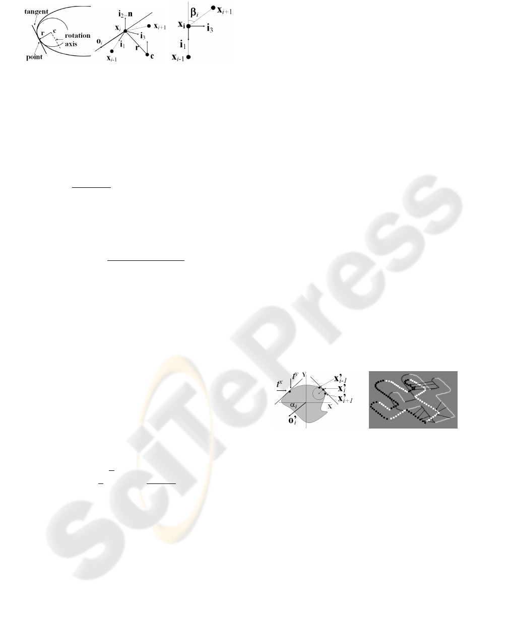
Figure 1: Local motor for a 3D contour (left). Local coor-
dinate system (middle) needed to get the circle parameters
of the motor and the structural features (right).
circle c and the radius vector r are easily calculated in
2D. Then the coordinates of the center of the circle in
3D are recovered. Thus, the rotation axis of the mo-
tor in 3D is obtained with the center c and the normal
vector n. The rotation angle θ
i
is the angle defined by
the segment
x
i−1
cx
i+1
. Finally the orientation vector
o
i
is defined by the orthogonal to the radius vector r
For every point of the 3D contour the local curva-
ture vector and bending angle are calculated by
k
i
= (x
i
− x
i−1
) ×(x
i+1
− x
i
)
β
i
= acos
(x
i
−x
i−1
)·(x
i+1
−x
i
)
k(x
i
−x
i−1
)kk(x
i+1
−x
i
)k
, (3)
where the points x
i
, x
i+1
and x
i−1
are considered in
the local coordinate system. In this case, the e
3
com-
ponent of the resulting curvature vector k
i
= x
1
e
1
+
x
2
e
2
+ x
3
e
3
changes its sign when the point is con-
cave or convex. When the scalar x
3
has a negative
sign, the point is considered locally convex. Other-
wise, it will be locally concave. If the bending angle
β
i
has a value closed to zero, the point is considered
as a part of a straight line.
An extended feature set allows to get more robust
features, especially in the image plane where noise is
present and digital contours are extracted. In this case
we are getting features not only from a single point.
The neighborhood of the point is extended to larger
segments in order to take average feature values as
shown in equation (4).
k
i
=
1
m
∑
m
j=1
v
1
× v
2
β
i
=
1
m
∑
m
j=1
acos
v
1
·v
2
kv
1
kkv
2
k
, (4)
where v
1
= x
i
− x
i−j
and v
2
= x
i+j
− x
i
.
By taking the point x
i
as a reference, motors
are constructed iteratively with the adjacent points.
Then the contour segment is defined by the points
{x
i−j
···x
i−1
, x
i
, x
i+1
···x
i+j
} and the features of that
point corresponds to the structure of the neighbor-
hood.
3.1 3d and 2d Contour Features
We define the following structural features for a 3D
point x
i
by
F
3D
i
= {o
i
, k
i
, β
i
}, (5)
where o
i
is the local orientation vector at the point x
i
,
k
i
is the curvature vector and β
i
the bending angle. To
get the corresponding 2D features, the contour model
points are projected onto the image plane ( see figure
2), motors are constructed and the features are cal-
culated as described in the last section with the cor-
responding points in image coordinates x
′
i−1
, x
′
i
and
x
′
i+1
. The normalized orientation vector o
′
i
is obtained
and its corresponding orientation angle α
i
.
The concept of phase in the image plane delivers
information of the local structure of the image derived
from the monogenic signal. In the case of edges, the
phase encodes a transition from one gray value to an-
other in x and y directions. For 3D contours it is not
possible to compute directly phase information in that
sense. Despite of that, it is possible to assign a fea-
ture value for a projected 3D contour point that rep-
resents such transition. We call this feature transition
index. Figure 2 shows the idea of transitions t
x
and t
y
for a point. The transition takes the values +1 or −1
(equivalent to the phase responses k r
x
i
k and k r
y
i
k)
depending on the orientation of the vector o
′
i
. Thus,
for a projected 3D contour point we obtain as features
the orientation and transition indexes in x and y direc-
tions F
con
i
= {α
i
, t
x
i
, t
y
i
} .
Figure 2: Example of motor construction and the transition
index in the image plane (left). Transition index of an pro-
jected model contour and phase response of the monogenic
signal (right). The lines show the corresponding pairs of
image and model.
4 STRUCTURAL ICP VARIANT
Our ICP variant combines error metrics with image
feature constraints. Thus, in the image plane we
have the following feature sets for projected model
segments F
2Dm
i
= {α
i
, t
x
i
, t
y
i
, k
2Dm
i
, β
2Dm
i
} and for de-
tected contour segments F
2Dp
i
= {φ
i
, k r
x
i
k, k r
y
i
k
, k
2Dp
i
, β
2Dp
i
}. Two points (image and model) form a
correspondence pair if the structural constraints are
met. The phase-transition index constraint is defined
as
C
1
=
1 if k r
x
i
k= t
x
i
∧ k r
y
i
k= t
y
i
0 otherwise
(6)
In the following we will use the sign ∧ to denote the
logical ”and” operation. The straightness constraint is
defined from the local bending angles β
2Dm
i
and β
2Dp
i
as
C
2
=
1 if β
2Dm
i
< t ∧ β
2Dp
i
< t
0 otherwise
, (7)
where t is a threshold value. Finally, the concavity-
convexity constraint is defined from the sign of the e
3
component of the vectors k
2Dm
i
= x
1
e
1
+ x
2
e
2
+ x
3
e
3
and k
2Dp
i
= y
1
e
1
+ y
2
e
2
+ y
3
e
3
by
C
3
=
1 if sign(x
3
) = sign(y
3
) ∧ C
2
= 0
0 otherwise
(8)
Figure 3: Example of correspondence pairs for normal (left)
and structural (right) ICP variants.
The figure 3 shows the idea of ICP combined with
structural constraints (straight, concave or convex).
The figure on the left shows the case where only the
minimal distance is considered, on the right for the
structural variant. As can be seen, for a point in
the bottom curve, its corresponding point in the up-
per curve will be the nearest point with the same lo-
cal structure. This is analogous for the ICP plus the
phase-transition index constraint, see left picture of
figure 2.
5 EXPERIMENTS
We used for our experiments 3D planar contour mod-
els (see figure 4) rich in structure like the ”cactus” and
”puzzle” models and also the ”mouse” model, which
has less structure. In the first experiment we compare
the convergence behavior of a normal ICP algorithm
and our structural ICP variant. The initial position of
the model is known, then it is translated and rotated to
its actual position and projected onto the image plane
to generate an artificial image. On this artificial im-
age the corresponding contour segments and the lo-
cal features are extracted. Then the pose is calculated
and compared with the ground truth. For these exper-
iments relatively large displacements were applied to
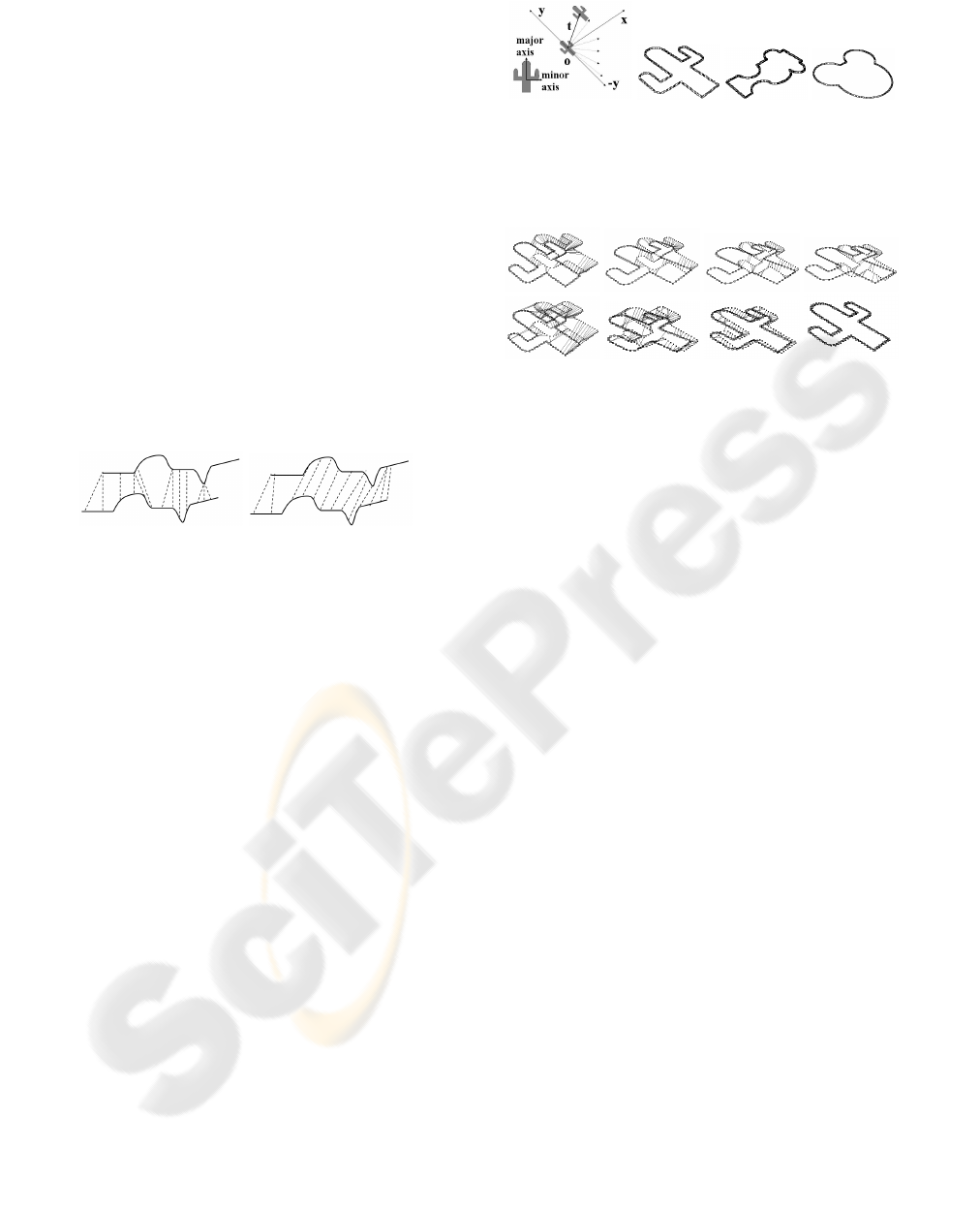
Figure 4: The object is translated in all directions in the
plane. For every translation the pose is calculated and com-
pared with the ground truth (left). Different models used in
the experiments (right): cactus, puzzle and mouse models.
Figure 5: Convergence sequence for normal (top row) and
structural (bottom row) ICP variants applied to the cactus
model.
the model in order to test the robustness against the
tracking assumption.
In the sequence of images in the figure 5, we com-
pare the convergence behavior of a normal ICP algo-
rithm against our structural variant when the tracking
assumption is not met. For such cases, the pose esti-
mation algorithm with the normal ICP variants does
not converge to the actual model position. A direct
comparison of the convergence behavior can be seen
in the the first row of figure 6. Two different pose
estimation algorithms were tested with our ICP vari-
ant, the 2D-3D (Rosenhahn and Sommer, 2005b) and
projective ones (Araujo et al., 1998). In both cases,
the structural ICP variants needs less iterations to con-
verge.
The normal variants of the ICP algorithm consider
as a correspondence constraint only the Euclidean
distance plus a weighting error factor or a different
search strategy. This has the effect that, in the first
iterations many bad conditioned correspondences are
found and therefore the convergence is slower or in
some cases, the algorithm does not converge at all.
The structural variant will also consider the constrains
of equations (6), (8) and (7). This increases the prob-
ability to find better conditioned correspondences and
therefore the convergence rate of the algorithm is in-
creased.
A second experiment was made to test the robust-
ness of our algorithm against the tracking assumption.
For this case, the model was rotated around its z axis
for zero to 50 degrees. As can be seen in the second
row of figure 6, with the structural ICP algorithm the
pose error is minimal for rotations up to 30 degrees for
0 10 20 30
0
20
40
60
80
100
Iteration
Absolute error (mm)
2D−3D algorithm
Normal ICP
Structral ICP
0 5 10 15
0
5
10
15
Iteration
Projective algorithm
Normal ICP
Structral ICP
Absolute error (mm)
0 10 20 30 40 50
0
50
100
150
200
Absolute error (mm)
2D −3D algorithm
Normal ICP
Structral ICP
Rotation angle (degree)
0 10 20 30 40 50
0
5
10
15
Rotation angle (degree)
Absolute error (mm)
Normal ICP
Structral ICP
Projective algorithm
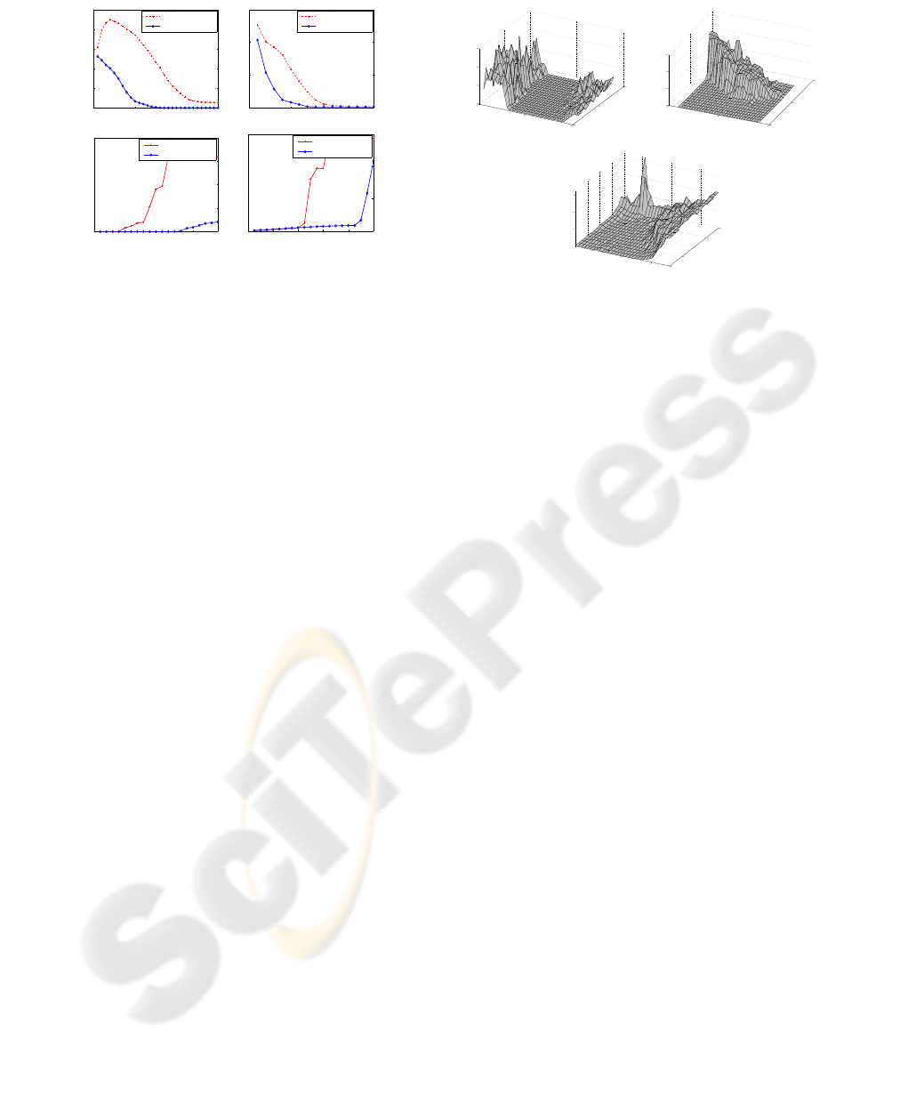
Figure 6: First row, convergence behavior comparisons of
the normal and structural ICP variants applied to the 2D-
3D pose estimation algorithm (left) and the projective algo-
rithm (right). Second row, robustness against rotations for
the 2D-3D (left) and the projective algorithms (right).
the 2D-3D algorithm and 40 degrees for the projective
one. This shows that our structural ICP variants al-
lows larger model rotations than the normal ICP vari-
ants. The robustness of the structural ICP algorithm
against the tracking assumption depends on the na-
ture of the object and its contour. For contours which
are rich in structural information larger rotations and
translations are allowed.
The next experiment was made to test the mag-
nitude and direction of the maximal possible transla-
tions allowed for the ICP structural algorithm. In this
case, as can be seen in figure 4, the object model was
translated to all directions in the plane where it is de-
fined. For every position the pose was calculated with
the structural ICP algorithm and the projective pose
estimation (Araujo et al., 1998).
The results for the cactus, puzzle and mouse mod-
els are shown in figure 7. These figures show the con-
vergence regions of the algorithm when translations
are applied. For the cactus, the algorithm is more sen-
sitive to translations in y direction, which corresponds
to translations in the major axis direction (see figure
4), while relatively large translations are allowed in x
direction (minor axis direction). The same effect can
be seen for the puzzle model. The figures show that
for certain positions the correspondence search is bet-
ter conditioned. As the translation increases, the prob-
ability to find more bad conditioned correspondences
also increases and therefore the pose error. The puz-
zle model and the cactus are complex objects, with
enough structure to deal with relatively large trans-
lations. The bottom figure shows the result for the
mouse model. In this case the mouse model does not
have much structural information. Therefore, as can
be seen in the figure 7, for large translations the error
0
50
100
−100
0
100
0
5
10
15
Translation in X
(mm)
Pose error for the translation case
Translation inY
(mm)
Pose error (mm)
0
50
100
−100
0
100
0
5
10
15
Translation in X
(mm)
Pose error for the translation case
Translation in Y
(mm)
Pose error (mm)
0
20
40
60
80
−50
0
50
50
100
150
Translation in X
(mm)
Pose error for the translation case
Translation in Y
(mm)
Pose error (mm)
Figure 7: Pose error for the translation case for the cactus
model (top left), for the puzzle model (top right) and for the
mouse model (bottom).
increases considerably.
Finally, we applied our algorithm to image se-
quences of a real scenario. The algorithm was tested
on a Linux based system with a 3 Ghz. Intel Pentium
4 processor. Some examples of the test sequences are
shown in the figure 8. The left column shows the ini-
tial position of our model and the right column the
pose result using our ICP structural variant and the
projective pose estimation algorithm. For every im-
age the monogenic signal response was obtained and
a contour search algorithm based on the local orien-
tation and phase information was applied to detect
the edge segments, then from these detected contour
points the structural features were calculated. The av-
erage computing time per frame, for the hole image
processing module, was 225 milliseconds. Due to the
relatively large displacement of the object, more iter-
ation steps are needed for the algorithm to converge
and therefore the computational time increases. For
these sequences the average computation time (image
processing plus pose estimation) was 2.65 seconds.
6 CONCLUSIONS AND FUTURE
WORK
A new variant of the ICP algorithm for pose estima-
tion of 3D free-form contours based on local struc-
tural model and image features was presented. The
experimental test proved that our structural ICP algo-
rithm performs efficiently for rich structured objects,
for large translations and rotations between scene and
object model. The experiments show that our ICP
algorithm combined with the projective pose estima-
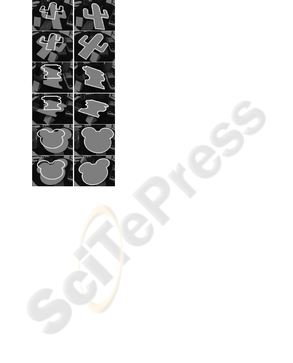
Figure 8: Initial position (left images) and estimated pose
(right images) for the cactus, puzzle and mouse model.
tion approach can handle larger object displacements.
That means, the feature constraints used to search cor-
respondences and the pose estimation constraints in-
volved in the minimization problem are better con-
ditioned in the image plane. Although our approach
does not reach requirements for real time applica-
tions (Rusinkiewicz and Levoy, 2001), the computa-
tion times reported for the test sequences are a good
tradeoff if we consider that the tracking assumption
has been significatively overcome. A natural exten-
sion for our approach is to consider the pose estima-
tion of non-planar free-form contours and surfaces
and to combine local and global structural features
(from model and image) to develop an approach capa-
ble to deal with even larger translations and rotations.
REFERENCES
Araujo, H., Carceroni, R., and Brown, C. (1998). A
fully projective formulation to improve the accuracy
of Lowe’s pose-estimation algorithm. Comput. Vis.
Image Underst., 70(2):227–238.
Benjemaa, R. and Schmitt, F. (1997). Fast global regis-
tration of 3d sampled surfaces using a multi-z-buffer
technique. In NRC ’97: Proceedings of the Interna-
tional Conference on Recent Advances in 3-D Digital
Imaging and Modeling, page 113, Washington, DC,
USA. IEEE Computer Society.
Besl, P. and McKay, N. (1992). A method for registration
of 3-d shapes. IEEE Transactions on Pattern Analysis
and Machine Intelligence, 14(2):239–256.
Chen, Y. and Medioni, G. (1992). Object modelling by reg-
istration of multiple range images. Image Vision Com-
put., 10(3):145–155.
Dorai, C., Weng, J., and Jain, A. (1997). Optimal registra-
tion of object views using range data. IEEE Trans-
actions on Pattern Analysis and Machine Intelligence,
19(10):1131–1138.
Felsberg, M. and Sommer, G. (2001). The monogenic
signal. IEEE Transactions on Signal Processing,
49(12):3136–3144.
Felsberg, M. and Sommer, G. (2004). The monogenic scale-
space: A unifying approach to phase-based image pro-
cessing in scale-space. J. Math. Imaging Vis., 21(1):5–
26.
Kass, M., Witkin, A., and Terzopoulos, D. (1987). Snakes:
Active contour models. International Journal of Com-
puter Vision, 4(1):321–331.
Rosenhahn, B., Brox, T., Cremers, D., and Seidel, H.
(2006). A comparison of shape matching methods for
contour based pose estimation. In 11th International
Workshop on Combinatorial Image Analysis (IWCIA).
Berlin, Germany, LNCS Springer-Verlag.
Rosenhahn, B., Perwass, C., and Sommer, G. (2004). Free-
form pose estimation by using twist representations.
Algorithmica, 38:91–113.
Rosenhahn, B. and Sommer, G. (2005a). Pose estimation
in conformal geometric algebra, part I: The stratifica-
tion of mathematical spaces. Journal of Mathematical
Imaging and Vision, 22:27–48.
Rosenhahn, B. and Sommer, G. (2005b). Pose estimation in
conformal geometric algebra, part II: Real-time pose
estimation using extended feature concepts. Journal
of Mathematical Imaging and Vision, 22:49–70.
Rusinkiewicz, S. and Levoy, M. (2001). Efficient variants
of the ICP algorithm. In Proceedings of the Third Intl.
Conf. on 3D Digital Imaging and Modeling, pages
145–152, Quebec City, Canada.
Shang, L., Jasiobedzki, P., and Greenspan, M. (2005). Dis-
crete pose space estimation to improve ICP-based
tracking. In 3DIM ’05: Proceedings of the Fifth In-
ternational Conference on 3-D Digital Imaging and
Modeling, pages 523–530, Washington, DC, USA.
IEEE Computer Society.
Sommer, G., editor (2001). Geometric Computing with Clif-
ford Algebras. Springer-Verlag, Heidelberg.
Zhang, Z. (1994). Iterative point matching for registration
of free-form curves and surfaces. Int. J. Comput. Vi-
sion, 13(2):119–152.
