IMPROVEMENT OF DEBLOCKING CORRECTIONS ON FLAT

AREAS AND PROPOSAL FOR A LOW-COST

IMPLEMENTATION

1,2

Frederique Crete,

Marina Nicolas

STMicorelectronics,12 rue Jules Horowitz, 38019 Grenoble, France

Patricia Ladret

Laboratoire des Images et des Signaux, 46 Avenue Félix Viallet, 38031 Grenoble, France

Keywords: Deblocking, flat areas, grey level gradation, low-cost, objective metrics.

Abstract: The quantization of data from individual block-based Discrete Cosine Transform generates the blocking

effect estimated as the most annoying compression artefact. It appears as an artificial structure caused by

noticeable changes in pixel values along the block boundaries. Due to the masking effect, the blocking

artefact is more annoying in flat areas than in textured or detailed areas. Existing low-cost algorithms

propose strong low-pass filters to correct this artefact in flat areas. Nevertheless, they are confronted to a

limitation based on their filter length. This limitation can introduce other artefacts such as ghost boundaries.

We propose a new principle to detect and correct the boundaries on flat areas without being limited to a fix

number of pixels. This principle can be easily implemented in a low-cost post processing algorithm and

completed with other corrections for perceptible boundaries on non-flat areas. This new method produces

results which are perceived as more pleasing for the human eye than the other traditional low-cost methods.

1 INTRODUCTION

The quantization of data from individual block-

based Discrete Cosine Transform generates the

blocking effect estimated as the most annoying

compression artefact. The blocking artefact appears

as an artificial structure caused by noticeable

changes in pixel values along the block boundaries.

Sometimes masked by textured areas, the block

boundaries are particularly detected by the human

eye on homogeneous or flat areas.

The blocking effect is well known and lots of

corrections have been proposed. Among them,

methods based on wavelet representation (Gopinath,

1994), on the Markov random fields, or on

projection on convex set (Yang, 1995), need high

computation time and memory. For real-time videos

processing, methods such as adaptive filters are

more suitable. However, some of these methods are

limited because they need to know the DCT

coefficients (Chou, 1998) or the information coming

from the decoder such as the quantization parameter

(List, 2003). To cover the largest possible domain,

we target our study to a post-processing deblocking

with the pixels value as the only aFvailable input

data. In this case of post-processing real-time

corrections, possibilities are limited and existing

algorithms are generally divided into two steps

(Kuo, 1995): a first step to localize the perceptible

boundaries and a second step to suppress these

boundaries. The detection step is made by an

analysis of the pixels values on both sides of the

boundaries. Then, according to this local pixel

information around the block boundary, an adaptive

filter is chosen for the correction step.

Unfortunately, this kind of correction has a

limitation due to the risk of overlapping between

input data to be corrected in current block and

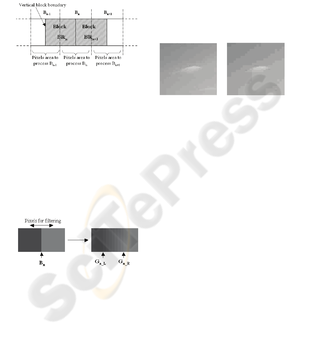
already corrected data from previous block. Figure 1

illustrates this phenomenon and shows that the

number of pixels used to process the detection and

the correction step is limited to the half length of a

block. For example, to correct the boundary B

n+1

, we

need to analyse the block Blk

n+1

which can has been

Crete F., Nicolas M. and Ladret P. (2007).

IMPROVEMENT OF DEBLOCKING CORRECTIONS ON FLAT AREAS AND PROPOSAL FOR A LOW-COST IMPLEMENTATION.

In Proceedings of the Second International Conference on Computer Vision Theory and Applications - IFP/IA, pages 32-39

 SciTePress

modified during the correction of the boundary B

By using the half length of the block, existing

algorithms avoid the phenomenon of overlapping

between two consecutive processes.

Figure 1: Traditional method to process a boundary.

After compression, flat areas are represented by

several homogeneous blocks. For a perceptible

boundary between two homogeneous blocks, the

major consequence of the limitation described above

is the apparition of two ghost boundaries on both

side of the initial boundary at the start and the end

positions of the correction. Figure 2 illustrates this

problem. Even if these ghost boundaries are less

perceptible than the initial one, they remain an

artificial structure which is annoying for the eye.

Averbuch et al (2005) propose to solve the problem

of ghost effect in flat areas using an iterative

principle based on varying size filters but still

limited to a size of eight. Even if this method has a

good performance, we focus our study on a non-

iterative and more simple method based on a simple

observation: the ghost boundaries disappear if the

correction is done on all pixels of the blocks.

Figure 2: The ghost boundaries G

n_L

and G

n_R

after

filtering the initial boundary B

In case of high compression rates, data are so

compressed that pixels value of homogenous blocks

converge to the same one. Consequently, in flat

areas, homogeneous blocks merge and form a larger

uniform block without intermediate boundaries.

Figure 3 shows that for high compression rates, there

are less boundaries but they are more perceptible. If

the boundaries are more perceptible, we can imagine

that the ghost boundaries made by a correction on a

fixed number of pixels will be highly perceptible

and very annoying for the eye. This phenomenon of

block merging has already been taken into account

(Pan, 2004) to refine quality metrics for high

compression rates. In the same way, if we localize

invisible boundaries caused by the block merging,

we will have more pixels available and we could

apply a stronger correction in order to avoid the

ghost boundaries apparition.

Figure 3: On the left, compression at 0.6 bbp, on the right,

compression at 0.4 bpp: for high compression, they are

less boundaries but highly perceptible.

By using the maximum number of pixels available

to correct a perceptible boundary, we propose a new

solution to remove the blocking artefacts on flat

areas without creating ghost boundaries.

In section 2, we explain our methods a) to

detect boundaries between two homogenous blocks,

b) to find invisible boundaries caused by the block

merging phenomenon and c) to explain the ideal

adaptive filter to correct these boundaries. In section

3, we describe how to implement these methods in a

low-cost algorithm by taking into account the

phenomenon of overlapping. Section 4 illustrates the

improvements on experimental results. Section 5

provides the conclusion of this paper.

2 METHODS TO DETECT AND

CORRECT THE BLOCKING

ARTEFACT ON FLAT AREAS

We consider the case of boundaries localized on a

regular 8x8 grid because digital video compression

algorithms like MPEG-1, MPEG-2 or H263 use a

size of block of 8x8 pixels. Our principle could be

easily adapted for a size of blocks of 8*4 or 4*4

pixels for compression algorithms like MPEG4 or

H264 but in the case of a shift grid due to a resizing,

a step to detect the boundaries position would be

necessary. We illustrate our purposes only on the

vertical boundaries but the principle is the same for

the horizontal boundaries.

IMPROVEMENT OF DEBLOCKING CORRECTIONS ON FLAT AREAS AND PROPOSAL FOR A LOW-COST

IMPLEMENTATION

2.1 Detection of Boundaries between

Two Homogeneous Blocks

To detect a boundary between two homogenous

blocks, we analyse the content of the blocks areas on

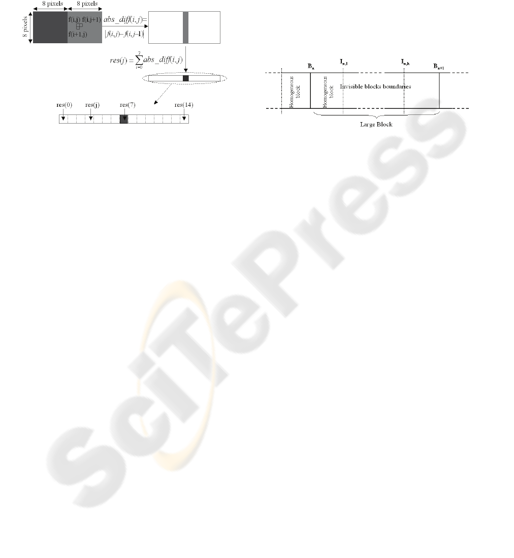
both side of the boundary. Figure 4 illustrates the

detection steps.

Figure 4: Detection of a boundary between two

homogeneous blocks.

step: On each line of the array f which represents

a pair of blocks, we make the absolute difference

abs_diff between neighbouring pixels to distinguish

flat from textured areas.

step: Then, by summing up the results over the

lines for each column, we are able to analyze the

global visibility of the boundary between two

blocks.

The left area is a homogeneous block if:

∑

0)(

jresLeftArea

(1)

The right area is a homogeneous block if:

∑

0)(

jresRightArea

(2)

The boundary is perceptible if:

TresholdresBound <=< )7(0

(3)

Over a range, the boundary is too perceptible to be

an artefact compression that is why the threshold is

used to not confuse the block boundaries with the

edges of the image content.

Finally, a boundary is defined as a perceptible one

between two homogeneous blocks if:

0=LeftArea

0=RightArea

TresholdBound<<0

(4)

2.2 Detection of Invisible Boundaries

Due to the Merging Block

Phenomenon

As we explain in the introduction, the large block

phenomenon is the result of a high compression:

neighbouring blocks merge and intermediate

boundaries become invisible. Consequently, the

major challenge to detect the large blocks without

intermediate boundaries consists in not confusing

them with the homogeneous regions of the initial

frame. To be considered as an invisible boundary

due to the merging blocks phenomenon, this

boundary must be in a highly compressed region.

Consequently, we define a large block (Figure 5) as

one or several invisible boundaries I

n,k

following a

perceptible boundary B

between two homogeneous

blocks.

Figure 5: The large block definition.

To detect an invisible boundary between two

homogeneous blocks, we use the same analysis as

the previous section (See Figure 4). We declare a

boundary invisible between two homogeneous

blocks if:

LeftArea

RightArea

Bound

(5)

Then, we declare that the invisible boundaries I

n,k

result from the block merging if:

is a perceptible boundary between two

homogeneous blocks

n,1

…. I

n,k

are invisible boundaries

(6)

2.3 Correction of Boundaries between

two Homogeneous Blocks

A boundary between two homogeneous blocks is

perceptible because the grey level g

left

of the left

block and the grey level g

right

of the right block are

different. Existing corrections are limited because

the absolute difference between g

left

and g

right

could

be so high that a filter on eight pixels is not

sufficient and can introduce ghost boundaries.

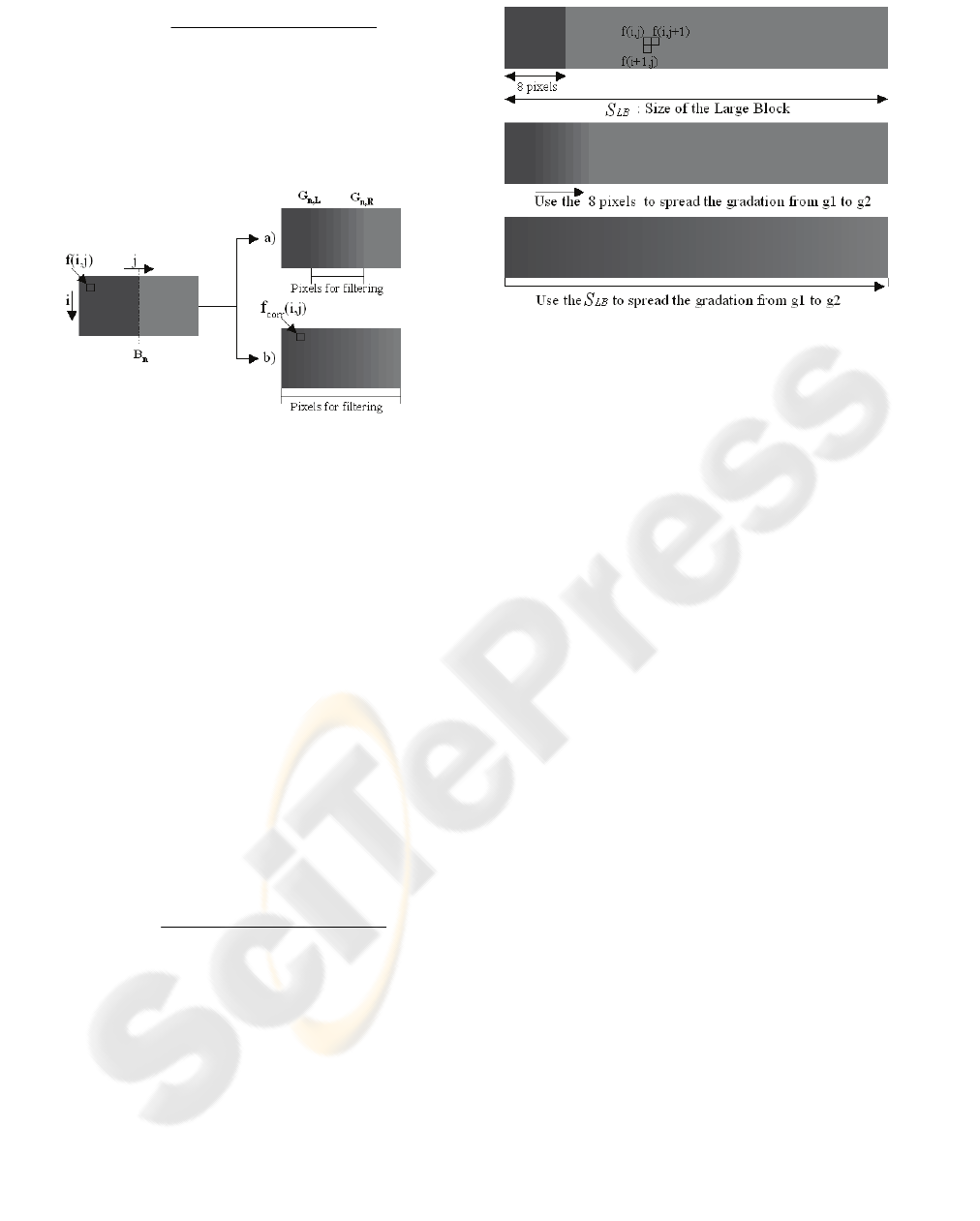
We propose a correction which consists in spreading

the gradation defined by the absolute difference

between g

left

and g

right

on the maximum number of

available pixels. This correction is introduced by the

equation (7) where f

corr

(i,j) is the correction of each

pixel (i,j) of the two adjacent blocks, S

is the size of

available pixels (16 in case of blocks of 8*8 pixels)

and g

left

and g

right

are the respective grey levels of the

left and the right blocks.

for j=0 to (S

-1) and for i=0 to 7:

VISAPP 2007 - International Conference on Computer Vision Theory and Applications

)1(

))1((

),(

−

×+×−−

rightleftB

corr

gjgjS

jif

(7)

Figure 6 shows the result obtained by using a) a

correction limited on a fixed number of pixels and b)

our correction. We observe that ghost boundaries

n,L

and G

n,R

have disappeared and the gradation

between g

left

and g

right

is better

spread.

Figure 6: Correction of a boundary using a) method

limited on the half length of a block b) method using the

entire blocks.

2.4 Correction of Boundaries Using the

Large Block Detection

The more the compression rate increases, the more

the absolute difference between g

left

and g

right

is high

and the more we need available pixels to spread the

gradation. By detecting the invisible boundaries

following a perceptible boundary (the block merging

phenomenon), we dispose to more available pixels

to spread the correction. The process until now

limited to 16 pixels can be extended to a number of

pixels proportional to the number of invisible

boundaries. The correction is traduced in the

equation (8) where S

is the size of the large block.

for j=0 to (S

-1) and for i=0 to 7:

)1(

))1((

),(

−

×+×

−

rightleftLB

corr

gjgjS

jif

(8)

Figure 7 shows the real improvement of the correction

when we use all available pixels compared to the

corrections limited to a fixed number of pixels.

Figure 7: Correction of a boundary using traditional

method limited on the half length of a block and our

method filtering on all available pixels.

3 PROPOSAL FOR A LOW-COST

IMPLEMENTATION

We propose in this section to include our methods

of detection and correction in a low-cost algorithm

able to take into account the overlapping

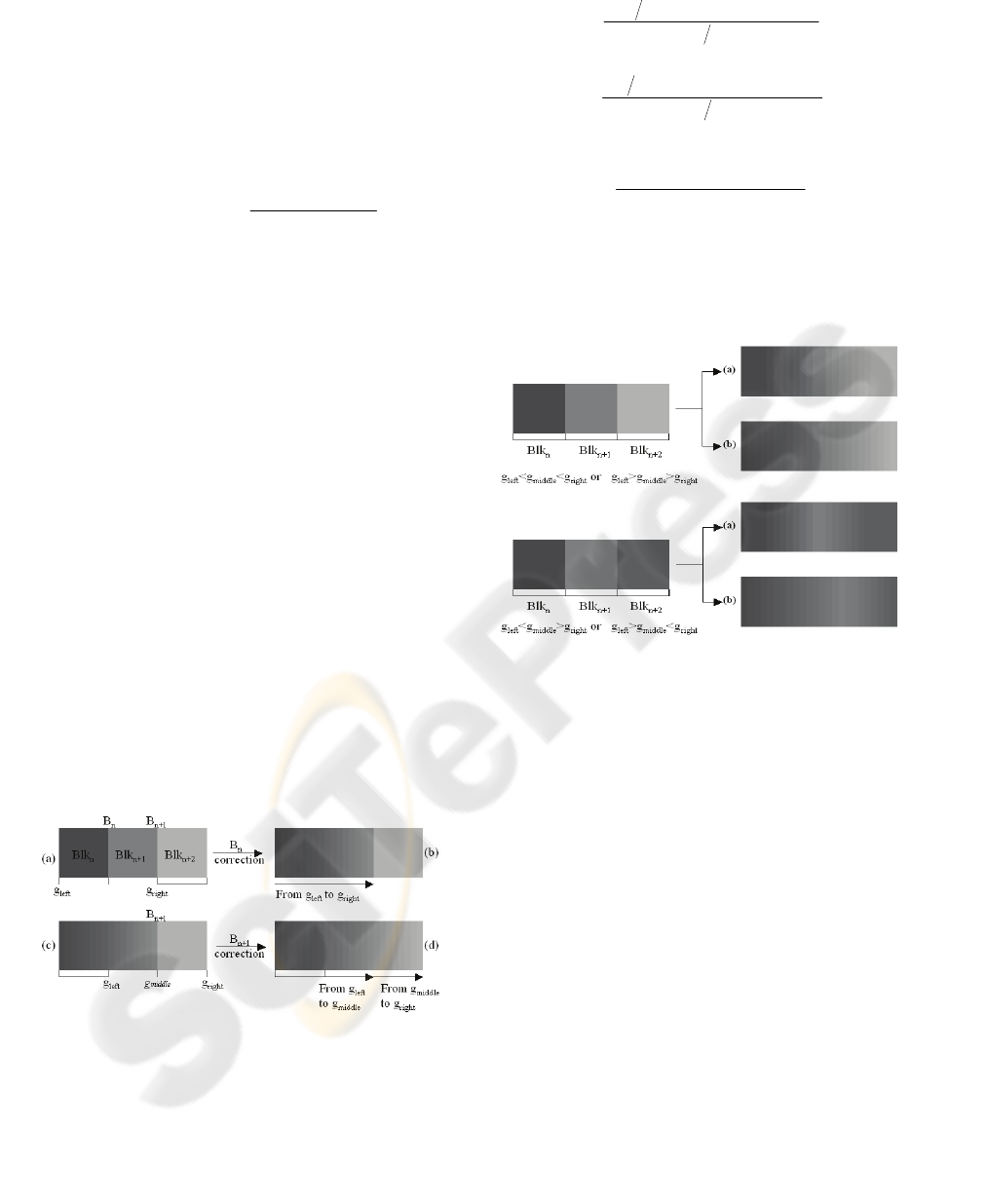
phenomenon. Figure 8 illustrates the steps presented

in the subsections 3.1 and 3.2.

3.1 Avoid the Overlapping Problem for

the Boundaries Detection

We consider Blk

as the left block, Blk

n+1

as the right

block and B

the boundary between Blk

and Blk

n+1

We suppose that the boundary B

is a perceptible

one between the two homogeneous blocks Blk

and

Blk

n+1

(Figure 8a). In this case, we apply a correction

on all available pixels using the equation (7). We

obtain the two corrected blocks Blk

and Blk

n+1

(Figure 8b). Moreover, we indicate into a flag that

the corrected boundary B

was a perceptible one

between two homogeneous blocks. To correct the

next boundary, the algorithm makes a switch of one

block. In this way, the algorithm studies the

boundary B

n+1

between the block Blk

n+1

and the

block Blk

n+2

(Figure 8c). If Blk

n+2

is an homogenous

block, we look for the flag. If the flag indicates that

the last correction was between two homogeneous

blocks, we know that before the last correction,

Blk

n+1

was homogenous. So, we have to consider

Blk

n+1

and Blk

n+2

as two homogeneous blocks. The

next step consists in computing the visibility of the

boundary so we have to compute the variable Bound

(3). Bound is the result of the absolute difference

IMPROVEMENT OF DEBLOCKING CORRECTIONS ON FLAT AREAS AND PROPOSAL FOR A LOW-COST

IMPLEMENTATION

between the last column of Blk

n+1

and the first

column of Blk

n+2

. Even if the pixels of the block

Blk

n+1

have been modified during the last correction,

our correction has not changed the last column of

Blk

n+1

Before the correction:

rightn giBlk =+ )7,(1

By applying the equation (7), we obtain the

correction:

right

rightleft

corrn g

ifiBlk =

×+×

==+

150

)15,()7,(

The compute of Bound is not biased by the

correction made on the 16 pixels.

The value of Bound reveals now if the boundary

n+1

is perceptible or not.

3.2 Avoid the Overlapping Problem for

the Boundaries Correction

To continue the previous example, we will see how

we take into account the overlapping problem for the

correction step.

3.2.1 The Boundary B

n+1

is Perceptible

If B

n+1

is detecting as a perceptible boundary

between two homogenous blocks (4), we apply the

equation (7) to spread the gradation between the new

left

and g

right

(Figure 8d).

But we have to slightly modify the equation to be

sure to represent all grey levels of the initial blocks.

In fact, if g

left

middle

right

or g

left

middle

right

, there

is no problem because to spread the gradation

between g

left

and g

right

, we meet g

middle

. But if

left

middle

right

or g

left

middle

right

, g

middle

would be

not represented.

Figure 8: Successive corrections of perceptible boundaries

between homogeneous blocks.

Consequently, we modify the equation by adding the

intermediate grey level g

middle

for i=0 to 7:

If g

left ≠

middle

or g

middle ≠

right

(9)

for j=0 to S

/2-1

))12((

),(

−

×+

−

middleleftB

corr

gjgjS

jif

for j=0 to S

/2-1

))12(

),(

−

×+

−

rightmiddleB

corr

gjgjS

jif

else

for j=0 to S

-1

)1(

))1((

),(

−

×+

−

rightleftB

corr

gjgjS

jif

end

Figure 9 illustrates the two cases corrected with

a)methods limited on a fixed number of pixels and

b)our method. We observe that our method does not

introduced ghost boundaries and make a better

gradation of all grey levels.

Figure 9: Correction of successive boundaries using a)

method limited on the half length of a block b) method

using the entire blocks.

3.2.2 The Boundary B

n+1

is Invisible

We suppose now that B

n+1

is detected as an invisible

boundary between two homogenous blocks (5). To

be conform with our definition of a large block

(Figure 5), we have to look at the type of the

previous boundary to decide of the next step. If the

flag is equal to 0, it means that the previous

boundary was not between two homogenous blocks.

The flag stays at 0 and there is no correction. On the

contrary, if the flag is equal to 1, we understand that

the last boundary was a perceptible one between two

homogeneous blocks. In this case, we define B

n+1

the first invisible boundary I

n,1

of a large block

(Figure 10). We apply the correction of the equation

(7 or 9) to spread the gradation between g

left

and

right

VISAPP 2007 - International Conference on Computer Vision Theory and Applications

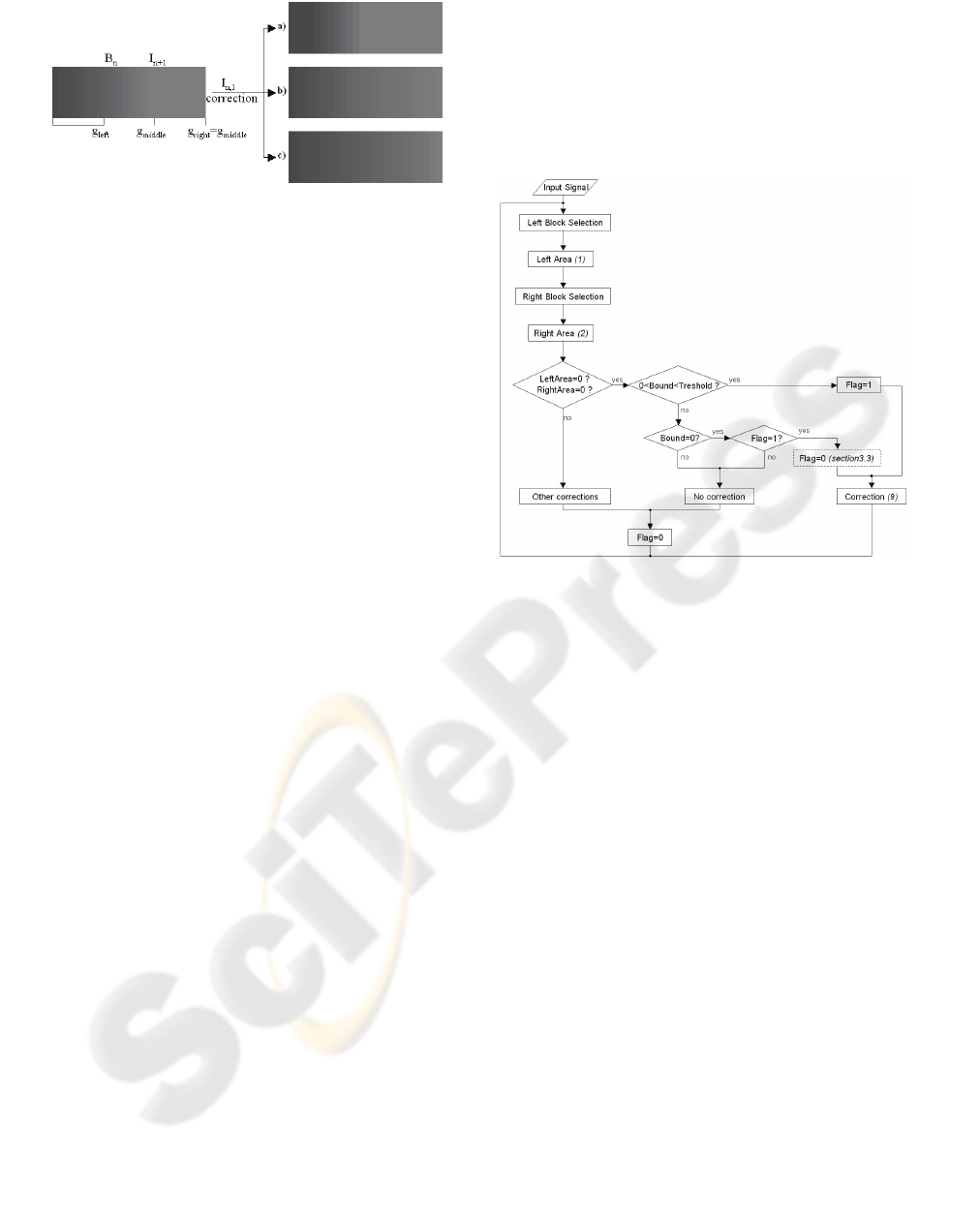
Figure 10: Large Block correction using a) method limited

on the half length of a block b) our principle in a low-cost

algorithm c) our principle.

This correction (Figure 10b) is slightly less

performed than the correction proposed in section

2.4 represented on Figure 10c. But we propose a

low-cost algorithm which make a one pass

processing on each pair of blocks. To apply the ideal

correction (section 2.4), we have to compute the

number of invisible boundaries and then to apply the

correction: this is impossible for a one pass

algorithm.

3.3 The Large Block Size

The threshold referred in the equation (3) of the

subsection 2.1 is used to distinguish an edge from a

block boundary. After several tests, we limited it to a

difference near from 24 grey levels. For this reason,

we estimate that a size of three blocks (24 pixels in

our case) is sufficient to make a good correction

without introduce ghost boundaries for a large block

correction. In this way, flag=0 after an invisible

boundary detection. Nevertheless, this number can

become insufficient for future implementation where

more than 8 bits would be used for the coding of the

pixel component values. In this case, the detection of

more than one invisible boundary can be useful.

3.4 Horizontal Boundaries and

Chrominance Component

In order to propose a low-cost algorithm, we do not

apply the large block correction for horizontal

boundaries. It is a means to avoid a complex control

of another variable flag for horizontal boundaries.

This limitation has not major consequences because

the large block is detected in most of cases on

homogeneous areas such as sky or sea where the

light has a tendency to be horizontally diffused.

In the same way, this kind of landscape has one hue

and variations are represented with the luminance

gradation. Consequently, the large block correction

is not necessary for the chrominance component.

3.5 Flow Chart of the Algorithm

To summarize those steps, we propose the flow chart

of this algorithm (Figure 11) with the sections and

the equations references. Moreover, we add in this

algorithm the possibility to combine other

corrections corresponding to perceptible boundaries

between textured or containing edges areas.

Figure 11: Flow Chart of the algorithm.

4 RESULTS

We propose to compare the results of “traditional

methods” which are low-cost algorithms based on a

fix number of pixels to “our method” which use all

available pixels. To represent the traditional

methods, we apply the same filter of our method but

only on four pixels on each side of the boundary.

This test is made for pictures with more or less flat

areas at different compression rates.

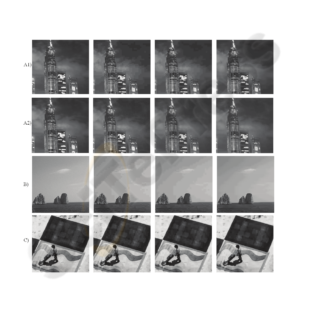
4.1 Visual Results

On Figure 12, we show from left to right the

uncompressed pictures, the compressed pictures,

pictures corrected with traditional method and

pictures corrected with our method. For the first

picture A1, the blocking artefact is very annoying.

Traditional methods correct the block boundaries but

we perceive again a blocking artificial structure due

to the ghost boundaries. Our method proposes a

correction perceived as more pleasing because it

does not introduce any new artificial block structure.

For the same picture A2 which is less compressed,

we have the same quality of results as the traditional

methods. We note for this picture that the initial

blocking artefact was not very annoying. For the

IMPROVEMENT OF DEBLOCKING CORRECTIONS ON FLAT AREAS AND PROPOSAL FOR A LOW-COST

IMPLEMENTATION

third picture B, we note the real improvement given

by our method. This picture has a large flat area that

is why our principle of correction is very suitable

(the correction would be better if we apply the

correction in the ideal case as we explain at the end

of the subsection 3.2.2). Then, the last picture C is

highly compressed but on small flat areas.

Consequently, the blocking artefact appears less

perceptible than on A1 or on B. We note that our

method is slightly better compared to traditional

methods, since the artificial structure of corrected

boundaries does not appear.

4.2 Objective Metrics

We analyse the results of our method with two

objective metrics. First, we use the traditional

PSNR. As the PSNR is a reference metric, we

compare the compressed and the two corrected

pictures to the original uncompressed picture.

Table1: PSNR resluts (dB).

Image Compressed

Traditional

Method

Our Method

A1 19,34 19,58 19,56

A2 19,34 21,11 21,12

B 20,17 20,28 20,28

C 24,09 24,47 24,46

Table 1 shows the benefit of the corrections with the

increase in PSNR values. Nevertheless, the PSNR

does not distinguish the two methods in term of

quality. This limitation is explained by the fact that

the PSNR is an algebraic measure for the quality of

the reconstruction of an image. In our case, a lot of

information has been lost during the compression

step and we try to obtain the reconstruction the more

pleasing for the human perception. In our case, the

PSNR is thus not well adapted.

Then, we confront the methods by using a no-

reference metric only focusing on the block

boundary visibility (Wang, 2002). This metric

ranges from 0 to 10 which are respectively the worst

and the best quality. As for the PSNR, the benefits

of the corrections appear in the results but this

metric does not distinguish the two methods either

(Table 2). We may infer that the Pan metric (Pan,

2004), which may be better adapted to our situation

thanks to its large block consideration, would give

scores for the compressed pictures that are better

correlated with the human perception. But this

metric will not distinguish the two methods either. In

fact, these methods measure the visibility of the

boundary on the initial grid position (every 8*8

pixels in most cases) that is why they are not able to

distinguish the improvement of our method. To give

an objective score of the visual improvement, we

have to use a metric able to localize all artificial

structures included the ghost boundaries.

Table 2: Wang metric results.

Image Original Compressed

Traditional

Method

Our

Method

A1 9,89

5,11 7,26 7,39

A2 9,89

7,82 8,32 8,38

B 9,67

5,14 7,54 7,59

C 10,13

4,48 8,11 8,21

5 CONCLUSION

We propose an algorithm able to improve the

deblocking correction on flat areas. The new

principle of our method is to use the maximum

number of available pixels to correct a perceptible

boundary. Using this method, we improve the

gradation between different grey levels without

introduce ghost boundaries. We focus our study only

on this artefact because it is very annoying for the

eye and experienced as the major principle limitation

of all traditional deblocking corrections. Our

algorithm is a low-cost one, thanks to the facts that

it is a one pass algorithm and that calculations used

to detect and correct the boundaries are very simple.

Visual results show the real improvement of our

algorithm on pictures containing flat areas and the

benefits of a large block correction for high

compression rates. Moreover, this principle can be

very favourable for future implementation where

more than 8 bits would be used for the coding of the

pixel component values. Finally, even if the visual

results show that our method gives results more

pleasing for the eye, we underline the difficulty to

characterize this perceptual improvement with

currently available objective metrics. These metrics

are not very well correlated with the human

perception because they do not take into account

other artificial structure such as ghost boundaries

which are also annoying for the human eye. Further

experiments are currently in progress to include this

new characteristic in an objective metric and to

correlate the results with subjective tests.

REFERENCES

Gopinath, R., Lang, M., Guo, H., Odegard, J. (1994).

Wavelet-based post-processing of low bit rate

transform coded images. Proc. IEEE Int.Conf. Image

Processing.

VISAPP 2007 - International Conference on Computer Vision Theory and Applications

Yang, Y., Galastanos, N.,Kastaggelos, A., (1995).

Projection-based spatially adaptive reconstruction of

block-transform compressed images. IEEE Trans.

Image Processing, vol. 4, pp.896-908.

Chou, J., Crouse, M., & Ramchandran, K., (1998). A

simple algorithm for removing blocking artefacts in

block-transform coded images; IEEE Signal

Processing Letters, vol. 5, pp. 33-35.

List, P., Joch, A., Lainema, J., Bjontegaard, G., &

Karczewicz, M, (2003). Adaptative Deblocking Filter

IEEE Transactions on Circuits and System for Video

Technology, vol. 13 , pp. 614- 619.

Kuo, C., Hsieh, R.J., (1995). Adaptive postprocessor for

block encoded images, IEEE Trans. Circuits Systems

Video Technology. vol5., pp 298-304.

Averbuch, A.Z., Schclar, A., Donoho, D., (2005).

Deblocking of Block-Transform Compressed Images

using Weighted Sums of Symmetrically Aligned

Pixels, IEEE Trans. on Image Processing, 14(2), 200-

212.

Pan, F., Lin, X., Rahardja, S., Lin, W., Ong, E., Yao, S.,

Lu, Z., Yang, X., (2004). A locally adaptive algorithm

for measuring blocking artifacts in images and videos,

Signal Processing: Image Communication19, pp. 499-

506.

Wang, Z., Sheikh H.R., Bovik, A.C., (2002). No-

reference perceptual quality assessment of JPEG

compressed images, IEEE International Conference

on Image Processing, pp. I-477-480.

Figure 12: From left to right: uncompressed picture, compressed picture, traditional methods, our method.

IMPROVEMENT OF DEBLOCKING CORRECTIONS ON FLAT AREAS AND PROPOSAL FOR A LOW-COST

IMPLEMENTATION