
FACE ALIGNMENT USING ACTIVE APPEARANCE MODEL
OPTIMIZED BY SIMPLEX
Y. Aidarous, S. Le Gallou, A. Sattar and R. Seguier
SUPELEC/IETR, Team SCEE, Avenue de la Boulaie BP 81127, 35511 Cesson Sevigne Cedex, France
Keywords:
Face alignment, Active Appearence Model, Nelder Mead Simplex.
Abstract:
The active appearance models (AAM) are robust in face alignment. We use this method to analyze gesture
and motions of faces in Human Machine Interfaces (HMI) for embedded systems (mobile phone, game con-
sole, PDA: Personal Digital Assistant). However these models are not only high memory consumer but also
efficient especially when the aligning objects in the learning data base, which generate model, are imperfectly
represented. We propose a new optimization method based on Nelder Mead Simplex (NELDER and MEAD,
1965). The Simplex reduces 73% of memory requirement and improves the efficiency of AAM at the same
time. The test carried out on unknown faces (from BioID data base (BioID, )) shows that our proposition
provides accurate alignment whereas the classical AAM is unable to align the object.
1 INTRODUCTION
In Human machine interface (HMI) it is necessary
to recognize objects (faces, hands, mouths) and an-
alyze them to identify motions and gestures. All of
these applications first need to align objects to be
recognized. We use Active Appearance Models to
align faces on embedded HMI (video phone, game
console). AAM was proposed by Edward, Cootes
and Taylor (G. J. Edwards, 1998) in 1998. They al-
low synthesizing an object with its shape and its tex-
ture. The AAM optimization proposed by Cootes in
(G. J. Edwards, 1998) was based on regression ma-
trix (RM). RM is capable of modifying parameters
to adjust model on an object. Taken of the avail-
able memory in on mobile technology the RM oc-
cupies a significant memory space, in order of many
Mega bits. We are going to use Nelder and Mead sim-
plex (NELDER and MEAD, 1965) so as to optimize
model parameters to reconstruct the face. The Nelder
and Mead simplex was used in face feature detec-
tion (Cristinacee and Cootes, 2004). Model of each
landmark (17 landmarks for face) is created and the
simplex optimize the placement of landmarks by us-
ing score function given by each model. The features
models are in low dimension compared by model of
whole face. (Cristinacee and Cootes, 2004) don’t op-
timize AAM parameters but placement of landmarks.
The simplex does not use prior knowledge, which
makes them efficient in generalization and they don’t
need too much memory space as well. The tests per-
formed, treat face alignment in generalization (learn-
ing data base from M2VTS (PIGEON, 1996), Test
data base from BioID (BioID, )). First we introduce
the classical AAM method and its different variant
proposed by community to find a solution reducing
required space memory (Section 2). In addition to that
we’ll present in section 3 the AAM simplex adapta-
tion, whereas generalization results are illustrated in
section 4 comparing to results obtained by classical
AAM. In section 5 we’ll conclude and present our fu-
ture works.
2 AAM: USED METHOD
In this section we’ll present classical AAM (G. J. Ed-
wards, 1998) optimized by RM and the problem come
across by this optimization. Subsequently, we’ll in-
troduce some method proposed by community to re-
duce required memory space for RM.
231
Aidarous Y., Le Gallou S., Sattar A. and Seguier R. (2007).
FACE ALIGNMENT USING ACTIVE APPEARANCE MODEL OPTIMIZED BY SIMPLEX.
In Proceedings of the Second International Conference on Computer Vision Theory and Applications - IU/MTSV, pages 231-236
Copyright
c
SciTePress

2.1 Classical Aam
AAM algorithm is constructed in two phases: The
learning phase in which we establish the model, and
the segmentation phase where we search the mod-
elized object in image.
2.1.1 Learning Phase
The learning phase generate mean model of object
from given data base. The shape of an object can be
represented by vector s and the texture (gray level)
by vector g. We apply one PCA on shape and another
PCA on texture to create the model, given by:
s
i
= ¯s+ Φ
s
∗b
s
g
i
= ¯g+ Φ
g
∗b
g
(1)
Where s
i
and g
i
are shape and texture, ¯s and ¯g are
mean shape and mean texture. Φ
s
and Φ
g
are vectors
representing variations of orthogonal modes of shape
and texture respectively. b
s
and b
g
are vectors repre-
senting parameters of shape and texture. By applying
a third PCA on vector b
b
s
b
g
we obtain:
b = Φ∗c (2)
φ is matrix of d
c
eigenvectors obtained by PCA. c is
appearance parameters vector. The modifications of c
parameters changes both shape and texture of object.
2.1.2 Segmentation Phase
The objective of this phase is to minimize error be-
tween segmented image and model by choosing pa-
rameters in order to align the model to this image.
To choose good parameters we need an optimization
method. In the case of classical AAM it has been done
with several experiments (by changing each variable
of parameter c). Each training data base object is an-
notated and represented with specific value of appear-
ance vector c and pose vector t, with the size d
t
, de-
fined by:
t =
t
x
t
y
θ S
T
(3)
Where t
x
and t
y
are x and y axis translation, θ is angle
of orientation and S is Scale. Let N be the number of
images, from the data base, of an object to align. Ob-
jects of training data base can be reconstructed from c
appearance vector which contain variations to add to
the mean model. Consider c
oi
, the value of c, which
represents object in the learning data base image i. By
modifying the parameter c
oi
in accordance with :
c = c
0i
+ δc (4)
we create new shape s
m
and new texture g
m
(For
example when we displace the model to the right,
we modify t by δt). The vector of error e
ik
is then
e
ik
= g
m
−g
0
,where k is the number of experiments
and g
0
is the texture of the data base image i under
the shape s
m
. Then we create experience matrix with
column representing experiment and row number of
pixels in a model (Eq. 5). A column of matrix G
(Eq. 5) is composed of a vector e
ik
. The linear re-
gression give us one linear relation between the gray
level error and pose parameter and another relation
between grey level error and appearance parameter:
T = R
t
G
C = R
c
G
(5)
C and T are the matrices where the modifications δc
and δt added to c
0i
and t
0i
(initial pose vector of object
in image i) at the time of each experiment. This gives
us the linear relation between δc and δt:
δt = R
t
∗δg
δc = R
c
∗δg
(6)
R
c
and R
t
are the appearance and pose regression ma-
trices respectively. δg is the gray level error on the set
of pixels constituting the object to align. The matri-
ces R
c
and R
t
allow us to predict the modifications of
c and t by having δg to align object. Regression ma-
trix optimization inducts drawback:
-Required memory : column number of regression
matrix is equal to number of model pixels. Row num-
ber is product of number of experiment q with the
number of parameter to be optimized: 4 for R
t
(Eq. 3)
and as much as parameter as eigenvector retained in
matrix φ (Eq. 2) for R
c
. RM size is important while
comparing the available memory in embedded tech-
nology.
The searching algorithm in new image is as follow:
1. Generate texture g
m
and form s according to c pa-
rameter (initially equal to 0).
2. Calculate g
i
, the image texture which is in the
form s.
3. Evaluate δg
0
= g
i
−g
m
and E
0
= |δg
0
|
2
4. Predict the modification δc
0
= R
c
∗δg
0
and δt
0
=
R
t
∗δg
0
which has to be given to the model.
5. Find the first attenuation coefficient k (among
1 0.5 0.25
) generate an error E
i
< E
0
,
with E
i
= |δg
l
|
2
= |g
m
−g
ml
| , g
ml
is the texture
create by c
l
= c−k ∗δc
0
and g
ml
is the texture of
image being in the form s
ml
(form given by c
l
.
6. if error E
i
is not stable, the difference E
i
−E
i−1
is
higher than a threshold ζ defined previously, re-
turn to step 1 and replace c by c
l
.
When the convergence is reached, the searching form
and texture face is generated with model given by g
m
and s represented using c
l
. The number of iterations
required is function of error E
i
stabilization.

2.2 Direct Appearance Model
This method (X. Hou and Cheng, 2001) is derived
from the classical AAM by eliminating the joint PCA
on texture (Eq.2) and form. It uses the texture infor-
mation directly for the prediction of the form: the es-
timation of position and appearance. It comes from
the fact that we could extract the form directly from
texture. The form and texture are built by PCA. The
main difference between the DAM and the AAM is
in the third PCA. We collect the difference between
the textures generated by small displacements in each
image of the training data base and by carrying out
a PCA on these differences so as to have a matrix of
projection H
T
. The difference in texture is projected
on under space such as:
δg
′
= H
T
∗δg (7)
The dimension of δg
′
present a quarter of the dimen-
sion of δg and the prediction is more stable. The re-
gression in the DAM then requires less memory than
the regression used in the AAM. The procedure of re-
search is the same one as the classical AAM except
for the prediction of the new form and texture. In [5]
it is shown that the size of the matrix of regression is
11, 83 lower than that of AAM.
2.3 Active Wavelet Networks
This method (Hu et al., 2003) uses the wavelets as
alternative to the PCA in order to reduce the dimen-
sion of space. It uses a Gabor Wavelet network (Hu
et al., 2003) to model the variations of the texture of
the training base. The GWN approach represents im-
age with a linear combination of functions of 2D Ga-
bor. The given weights are of the form to preserve the
maximum information contained in image for a fixed
wavelet number. The method of search of faces (or
unspecified object) is the same one as that of the clas-
sical AAM by disturbing the initial positions and to
put a linear relation (matrices of regressions) between
the displacement of the parameters and pixels error.
The DAM and AWN methods make it possible to
reduce the required memory to store RM. In the fol-
lowing section we propose a method to remove the
space allocated to store these matrices.
3 AAM OPTIMIZATION
We propose to use the Training part (Section 2.1.1),
by optimizing the search (Section 2.1.1) appearance
(Eq.2) and pose (Eq.3) parameters by using Nelder
Mead Simplex (SP)[2]. It is a numerical method of
optimization which will allow us to find solutions
minimizing pixels error. This method gives us the
possibility of converging in population (together of
solution convergent toward the same minimum) mak-
ing the solution more stable, to be direct: no cal-
culation of derivative and to converge in a number
of iteration which is rather tiny compared to another
global optimization methods requiring a great num-
ber of iteration like the Genetic Algorithms, Simu-
lated Annealing... They will also enable us to reduce
required memory used in classical AAM optimization
by preserving only the average model; we don’t have
to store RM.
3.1 Nelder Mead Simplex Algorithm
The simplex of Nelder Mead (NELDER and MEAD,
1965) makes it possible to find the minimum of func-
tion of several variables in an iterative way. For two
variables the simplex is a triangle and the method con-
sists of comparing the values of the function on each
top of the triangle. Thus the top where the function is
highest is rejected to be replaced by another top which
will be calculated according to the precedents. The
algorithm is called simplex considering the general-
ization of the triangle in n dimensions. The stopping
criterion of algorithm will be a threshold of the dif-
ference between the values of the function to be min-
imized given by the current solutions. This threshold
will determine number of iterations necessary to con-
verge. The error to be minimized is the pixels error
[Eq.11] used by the classical AAM.
For new solutions, all the operators of search base
themselves on a center of gravity x
c
=
1
n
n
∑
i=1
x
k
i
calcu-
lated compared to the current solutions in each iter-
ation and giving a direction d
k
= x
c
−x
k
n+1
worms
of the solutions minimizing the error function. Let
us note E the objective function to be minimized.
The operators of search for solutions minimizing this
function are as follows:
• The Reflection: we test the point which is in the
opposite direction of the bad solution:
x
r
= x
k
n+1
+ 2d
k
= 2x
c
−x
k
n+1
. (8)
• The Expansion: we prolong research beyond the
point of reflection by testing the solution:
x
e
= x
k
n+1
+ 3d
k
= 2x
r
−x
c
. (9)
• The Contraction: if the previous two operators of
search fail then we minimize tests points close to
share and other of the current solution:
x
−
= x
k
n+1
+
1
2
d
k
=
1
2
(x
k
n+1
+ x
c
)
x
+
= x
k
n+1
+
3
2
d
k
=
1
2
(x
r
+ x
c
)
(10)

• The Shrinkage: if all the preceding solutions do
not minimize E we narrow down the triangle by
changing these tops, and tests the preceding dis-
turbances.
3.2 Simplex Adaptation to Aam
We propose to adapt the Nelder Mead algorithm
(NELDER and MEAD, 1965) to optimize the AAM
parameters in segmentation phase. The minimized er-
ror is the sum of quadratic errors between real image
and generated model on each pixel:
E =
M
∑
i
e
2
i
(11)
A model is described by:
v =
c
t
(12)
Size of v is d
c
+ d
t
(d
c
and d
t
are the c (Eq. 2) and t
size (Eq. 3)), the simplex must optimize d
c
+ d
t
pa-
rameters to align the model on the face. The natural
way will be to optimize pose and appearance sepa-
rately like RM (Eq. 6) by implementing two simplex
one for pose and other for appearance. Single simplex
applied on set of parameter will be more efficient (In
quality of time and convergence). The simplex starts
search from d
c
+ d
t
+ 1 solutions chosen randomly in
space under constraint. So as to use the simplex al-
gorithm in AAM optimization, stopping criterion and
variables constraint must be defined.
Constraints: they are applied to avoid testing incor-
rect solutions that we know preliminary. These con-
straints bound search space on appearance and pose
variables. We initialize the vector v (Eq. 12), rep-
resenting appearance and pose, randomly in interval
corresponding to each parameter under Cootes’s con-
straint:
• Appearance constraint: appearance variable inter-
val is −2
√
λ et 2
√
λ (Stegmann, 2000). Where λ
is the eigenvalues of the eigenvectors correspond-
ing to matrix G
T
G, G is the gray level differ-
ence matrix between modifying model and real
image. These constraints are verified during al-
gorithm execution.
• Pose constraints: AAM is robust till 10% in scale
and translation (T. Cootes, 2002). We initialise
the pose variable (x and y axis translation, rotation
and scale) in the interval of 10% of the object real
pose vector.
Stopping criterion: the algorithm will end after fixed
number of iterations (to insure maximum processing
time) or when it will converge in population. The
population convergence is obtained if difference be-
tween the E values (Eq.11)of the proposed solutions
do not pass the threshold S
E
. In the case of error
normalization, done by Stegmann in (Stegmann,
2000), the mean value of the error is stable E
mean
on different images of the same object, at the time
when the alignment is correct. We propose to settle
S
E
= 0.1×E
mean
.
Simplexes neither need additional required mem-
ory space necessary to store the model nor informa-
tion on the directions to a priori to minimize the error
E. Typically the number of experiments necessary for
the training phase is 90 (4 for each appearance para-
meter and 6 for each pose parameter). The size of
the two matrices (of appearance R
c
and of pose R
t
)
is equal to M ×(d
c
+ d
t
) Bytes, M being the num-
ber of pixels contained in texture of the model. For
our test with images 64×64pixels the size of the re-
gression matrices (Eq. 5) is 86KB. The mean model
size is 33KB. The memory require for the AAM is
≈ 120KB. In the case of the simplex we don’t need
RM, therefore the memory used is 33KB. Memory
space required by the simplex is lower than that used
in (Hu et al., 2003) which memorizes the wavelet co-
efficients in addition to the model and also lower than
that needed in (X. Hou and Cheng, 2001).
4 RESULTS
To evaluate the performance of our proposed opti-
mization, we tested alignment of face in generaliza-
tion: the tests were realized on faces which not belong
to the training base. The training data base is made
up of 10 images belonging to the European data base
M2VTS (Multi Modal Checking for Teleservices and
Security applications; Fig.2)(PIGEON, 1996). Our
method was tested on images of the base BioID (bio-
metric Identity; Fig.3)(BioID, ). To qualify the con-
vergence of the AAM we will define an error of mark-
ing. This error f
i
(i = 1, 2, 3) was calculated for each
part of the face i = eyes, noise, lips such as:
f
i
= p
find
gi
− p
real
gi
avec : p
real
gi
=
1
Q
i
Q
i
∑
r=1
p
real
ir
et p
find
gi
=
1
Q
i
Q
i
∑
r=1
p
find
ir
(13)
p
real
ir
are the coordinates of the ground truth of the
points of marking of the i part of the face, p
find
ir
the
coordinates of the points of marking of the part of
the face i found by algorithm and Q
i
is the number
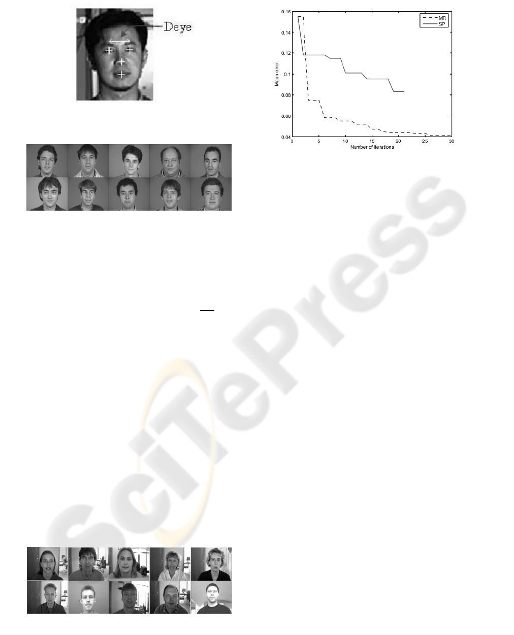
Figure 1: D
eye
distance.
Figure 2: Learning data base from M2VTS.
of point of marking of the i part. The algorithm con-
verges when the 3 errors were lower than convergence
threshold. The threshold was calculated according to
the distance between the eyes. In these tests we have
taken the threshold of convergence equal to
D
eye
5
(Fig.
1). That guarantees a rather precise convergence.
Number of iterations: In order to compare SP
optimization with that of RM, we need to fix the
minimum number of iterations needed by AAM to
converge. With this intention we have tested the
AAM on the 10 faces of BioID by fixing the number
of iteration at 30 for shift of t
x
= −4 pixels. Only
the images on which the AAM converged were taken
into the account. From it we deduce a curve of
convergence of the quadratic errors between pixels
(minimized error) from the successfully converged
images. The curve of figure 4 shows the number
of iterations required by AAM to converge, at the
bottom of an error of 0.05 the AAM have converged
with 18 iterations in our case. The average of curve
is made on the curves belonging to the images
where our algorithm have converged. The realized
curve of convergence compared to the number of
Figure 3: Test data base from BioID.
Figure 4: Mean of convergence curve of algorithm using
RM and SP.
iterations is shown in figure 4. The comparison of
the two curves shows that the error obtained by RM
(≈ 0.05) is lower than that found by SP ≈ 0.094.
The minimum of this error is not always a good
adjustment of the model on the true face in test image
and depends much on initialization. Even if the SP
found higher error, it presents better results in term
of marking error. That is illustrated in the figure 6.
The initialization has an influence on the minimum
of the function error reached by each algorithm of
optimization. Figure 7 presents the results obtained
by an initialization on the true face (t
x
= 0, t
y
= 0,
true scale
,
true orientation
) comparing
convergence in error of marking and pixels. It shows
that optimization by SP gives better results in terms
of pixels and marking in the case of a favorable
initialization.
Robustness on initialization: Knowing that our al-
gorithm convergesunder the same conditions (an even
number of error calculation), we plot the curve of con-
vergence expressed as a percentage of converged im-
ages compared to displacements in t
x
. So to remove
random aspect of SP initialization, we did 10 simplex
and we obtained mean curve of convergence. Figure
5 represents a comparison between the realized curve
and that obtained by RM.
Figure 5 shows also that SP optimization has same
capacities of convergence in the most favorable case
(the case where initialization is on the true face) while
having the same number of error calculation. The use
of Nelder Mead algorithm as an optimization method
of AAM allows being more robust than RM in term of
initialization. Even starting in far initialization we ob-
tain better results than the RM. The difficulty to align
unknown faces is caused by the initialization (Eq. 2).
In the learning phase the error is generated by c
0i
(true
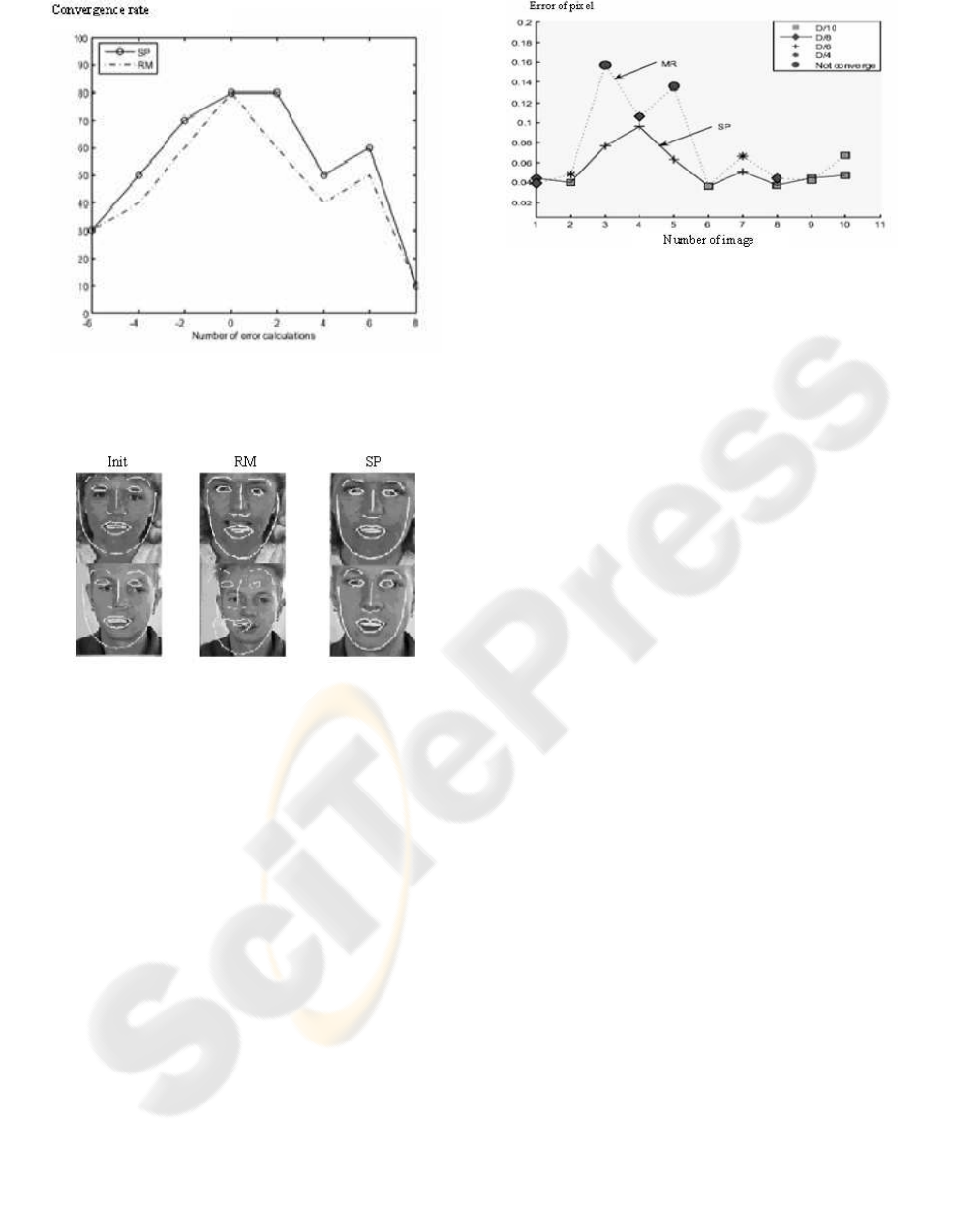
Figure 5: Comparison between convergence rate of RM and
SP in terms of marking error in different translation initial-
ization.
Figure 6: Results obtained on faces with RM (middle) and
SP (right).
face model parameters). In (Eq. 4) the new shapes are
generated from modifications of δc on vector repre-
senting the true face c
0i
. Whereas research in segmen-
tation phase is initialized by using mean shape and
texture. If faces contained in test data base are differ-
ent than faces belonging to learning data base, the RM
present difficulty to predict the appropriate modifica-
tions. In the case of the Nelder Mead optimization
there is several initialization which can converge to
the true face by non linear changes of solutions.
The results obtained in figure 6 show the capacity
of the SP to find solutions which converge toward the
true face while having a higher degree of accuracy
comparing with RM.
5 CONCLUSION
The reduction of necessary memory space on embed-
ded technologies required to use algorithms which are
Figure 7: Results obtained on faces initialized by t
x
= 0
using RM et SP by highlighting convergence by distance
D
eye.
greedy in the requirement data storage for system be-
havior. We proposed to use Nelder Mead algorithm
instead of RM optimization in the segmentation phase
of AAM. It allows us to save 73% of the memory used
by the classical AAM while being more robust in ini-
tialization compared to initialization of the model.
THANKS
This research was supported by Brittany Region (”re-
gion de bretagne”) in France.
REFERENCES
BioID. Biometric identity data base, www.bioid.com.
Cristinacee, D. and Cootes, T. (2004). A comparaison of
shape constrained facial feature detectors. pages 375–
380.
G. J. Edwards, C. J. Taylor, T. F. C. (1998). Interpreting
face images using active appearance models.
Hu, C., Feris, R., and Turk, M. (2003). Active wavelet net-
works for face alignment.
NELDER, J. A. and MEAD, R. (1965). A simplex method
for function minimization. volume 7, pages 308–313.
PIGEON, S. (1996). www.tele.ucl.ac.be.
Stegmann, M. (2000). Active appearance models theory,
extension and cases.
T. Cootes, P. K.-n. (2002). Comparing variations on the
active appearance model algorithm. pages 837–846.
X. Hou, Stan Z. Li, H. Z. and Cheng, Q. (2001). Direct
appearance models.
