COLOR CALIBRATION OF AN ACQUISITION DEVICE

Method, Quality and Results

V.Vurpillot, A.Legrand, A.Tremeau

Ligiv, Universite Jean Monnet, 18 rue Benoit Laurast, Saint Etienne, France

Keywords: Color calibration, spectral, sensitivity recovery, correction quality, reconstruction errors.

Abstract: Color calibrated acquisition is of strategic importance when high quality imaging is required, such as for

work of art imaging. The aim of calibration is to correct raw acquired image for the various acquisition

device signal deformation, such as noise, lighting uniformity, white balance and color deformation, due, for

a great part, to camera spectral sensitivities. We first present reference color data computation obtained from

camera’s spectral sensitivities and reflectance of reference patches, taken form Gretag MacBeth Color Chart

DC. Then we give a color calibration method based on linear regression. We finally evaluate the quality of

applied calibration and present some resulting calibrated images.

1 INTRODUCTION

This study presents a method of calibration for a

color acquisition system. Once the whole system has

been characterized, the next step consists in

calibrating this system to get data that are

independent face to all possible acquisition system

parameters evolution during the various acquisition.

In order to be able to carry out such a calibration

method, the color data which will stand as reference

for calibration must be determined. In this purpose,

the most accurate estimation of acquisition system

spectral sensitivity curves has to be performed. Error

computation from results of the various known

methods allows to select the method providing the

best results. This study describes some methods and

results.

Calibration methods can then be developed. We

present the established calibration method for our

system, with analysis on its quality, and on its

carrying out on some works of art.

Image acquisition process is known as

interaction between illumination spectral

distribution, object spectral reflectance and imaging

system characteristics. We denote the linearized

sensor response for the k

channel (R, G or B, or

monochrome) by C

, the linearization function by F,

the exposure time by e, the sensor noise for the k

channel by b

, the sensor spectral sensitivity function

for the k

channel S

(λ), by L(λ) the total incident

light on sensor (illumination * reflectance) and the

spectral range [λ

- λ

]. The camera response C

, for

an image pixel, is determined by equation (1).

()()

kk k

CFeS L b

λλ

λλλ

⎛⎞

=Δ+

⎜⎟

⎝⎠

∑

(1)

2 REFERENCE COLOR DATA

Our calibration aims to transform acquired raw RGB

data to a fixed and determined RGB space, in order

to get similar and comparable color data, whatever

the acquisition time, possible evolution in lighting

distribution and in system spectral sensitivity. Here,

the chosen RGB space is related to the system: it can

be obtained from system spectral sensitivity curves

and lighting spectral distribution. The reference

chart used for calibration is the Gretag MacBeth

Color Chart DC (240 patches). Thus, we first need to

know these patches’ RGB theoretical values in our

defined RGB space.

157

Vurpillot V., Legrand A. and Tremeau A. (2007).

COLOR CALIBRATION OF AN ACQUISITION DEVICE - Method, Quality and Results.

In Proceedings of the Second International Conference on Computer Vision Theory and Applications - IFP/IA, pages 157-160

 SciTePress

2.1 Recovering Spectral Sensitivity

The first step consists in finding the most accurate

spectral sensitivity curves of our acquisition system

(channel R, G and B).

A classification of the most common methods can be

given in two paradigms, indirect estimations and

direct measurement methods which we will not

detail here. Resulting curves are given for our

acquisition system.

Many indirect estimation methods have been

tested: by Pseudo-Inverse (Quan, 2003), by selecting

principal eigen vectors (Hardeberg, 2000), by adding

a smoothing constraint (Paulus, 2002), by mixing the

two precedents methods (Paulus, 2002), and by

combining basis functions, (Quan, 2003).

Another range of methods consists in finding

sensitivity curves by direct determination (Vora and

Farrell, 1997). We consider here camera responses

to narrowband sampling of illumination.

In order to estimate sensitivity reconstruction

validity and to select the one giving the most

accurate results, errors in reconstruction have to be

evaluated. This is achieved by estimating 540

patches P

from computed sensitivity curves (2).

()()

()

PSL

∑

(2)

Various error computations are made, such as

mean and maximum absolute and relative errors,

standard deviation and RMS, for each channel and

each of the recovered sensitivity curves.

A first analysis of computed errors leads us to

select one method of estimation and one direct

measurement method among all recovered curves.

Comparing both leads to conclusion that, although

methods are unconnected, error results are really

closed. As carrying out an estimation method is

faster, it will be kept rather than direct measurement.

The selected method is the one using smoothing

constraint. This curve is shown in Figure 1.

2.2 Theoretical Color Computation

From these sensitivity curves, theoretical patches

can be computed (equation 3). They will stand as

basis for color calibration. To get this theoretical set

of RGB patches (Patch

Theo,k

), a white balance

SysBal

is applied.

() ()

(

)

Theo k

Patch

SysBal

∑

(3)

-50 0

50 0

1000

15 0 0

2000

2500

3000

380 480 580 680 780

W aveleng t h( nm)

Sensit ivity

Figure 1 : Resulted Sensitivity curves estimation

It corrects system white deformation due to S

λ,k

while keeping the white relative to illuminant,

chosen such that color can be well rendered.

3 CALIBRATION

To calibrate the system, three acquisition steps are

required for correction. These corrections will also

be applied to chart acquisition itself, to get correct

mean values of acquired patches in order to calculate

transformation.

3.1 Calibration Steps

First acquisition consists in recording a dark image.

Let Im

obs

be this image. Next acquisition, Im

Unif,k

intends to correct lighting and system acquisition

non-uniformities (lens + RGB sensor), with a white

chart. This double correction is applied with

following equation (4), correction to which is added

white balance (described previously):

kobskUnif

obsk

kUnifkCor

SysBal

Ratio

ImIm

*Im

−

(4)

Ratio

Unif ,k

is chosen in such a way that the RGB

values of a pixel which coordinates correspond to a

maximum value in uniformity image, remain the

same.

The final calibration step consists in computing

color transformation. It will make possible to change

from acquired raw chart patches over theoretical

patches. In practice, numerous transformation

matrixes are computed for our calibration,

corresponding to different integration times,

determined from regularly sampling time range.

VISAPP 2007 - International Conference on Computer Vision Theory and Applications

158

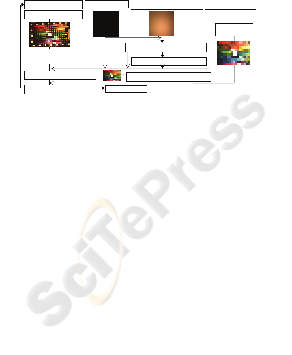
Figure 3 : Diagram of the different steps required to get RGB transformation for calibration

Once the chart acquired, it is corrected following

equation (4). Then, only “linear” mean value of the

patches set are kept for transformation computation:

the three R, G and B values of these patches must

stand in the sensor linearity range (above noise and

below saturation knee). The number of kept patches

is dependant of the considered integration time. All

steps are summed up in Figure 3.

3.2 Transformation Computation

Let Patch

Acqui,k

the acquired patches set, for a chosen

integration time. The transformation we obtained has

been selected among various methods, adapted from

Martin Solli’s methods (Solli, 2004). A linear

regression has to be performed.

The simple and general transformation is given

by equation (5):

)(

AcquiTheo

PatchgPatch =

(5)

An approximation of g-function can be

expressed by the following expression (6):

avPatchsg

Acqui

=)(*

(6)

with v the corresponding vectors of Patch

Acqui

(vector v is M functions h

(x) of Patch

Acqui

). Vector a

(M coefficients) which minimizes RMS difference

between acquired and theoretical data, is given by

the Moore Penrose pseudo-inverse resolution.

An important step then consists in choosing the

right parameters in v vector. We have tested many of

these parameters and the one we kept for our

calibration, after a similar study on errors than

previously, is the one called “combined order

polynomial regression” (Orava, 2004).

3.3 Quality Measurement

As observed previously, for each integration time

used for calibration, the number of kept patches

varies. We need to know if some criteria of quality

can be determined, in order to decide whether the set

of patches are representative of the color space or

not, and thus to validate calibration quality.

A first evaluation on patches is made on their

repartition in the camera RGB cube. This repartition

can be represented, as well as its projection on the

three different RG, GB and RB plans. An example

of it is given for two integration times, under a D65

lighting (figure 3). Same measurements have been

done under a other illuminant (halogen lighting).

For low integration times, patches projection is

concentrated in low values space: thus, this space is

precisely sampled, but not very representative of the

remainder of RGB cube. The more integration time

grows, the more RGB cube is represented by patches

(better under D65 lighting than under halogen

lighting), but coarser the sampling is and lower the

number of kept patches is (saturated patches

increasing). Statistics on relative and absolute errors

have been calculated, for various combinations of

calibration and patches.

For each test, error evolution is the same. At low

integration times, error is high. It then decreases

down to a floor, value which is kept during an

important integration time range. It finally

significantly grows for higher integration times.

Noise correction of uniformity chart

Noise acquisition

RGB acquisition of the white chart

RGB uniformity ratios computation

System white balance

Theoretical

atches

Chart RGB acquisition

Chart correction for noise,

uniformity and white balance

Mean patches computation

Transformation computation

End

Integration time selection

Calibration quality estimation

COLOR CALIBRATION OF AN ACQUISITION DEVICE - Method, Quality and Results

159

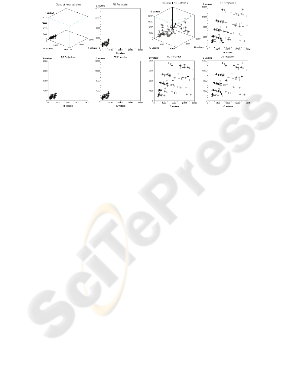
Figure 4 : Repartition of RGB patches in camera RGB cube, and on RG, RB, GB projection plans for

integration time of 62.5ms (right) and 500ms(left).

Considering that an error variation above 200%

of its lowest level, implies that this error is not

acceptable, for calibration with 170 patches, whether

being under D65 or under halogen illuminant, more

than 50% of the whole patches set have to be kept in

order to get R, G and B errors in this range.

The various results show that only considering a

number of patches is not sufficient. Criterion of

calibration quality also depends on lighting and

chart. Only knowing these conditions allows such a

criterion: for D65 lighting with a Gretag MacBeth

Color DC chart, calibration gives little errors, if the

number of kept patches, is higher than 50% of the

170 original patches.

Other aspects have to be taken into account: if

integration time is low, when considering patches

that are projected outside the restrained represented

volume, committed errors are then very high, as

those patches have not been taken into account when

calibration matrix has been computed.

4 CONCLUSION

Once calibration data are computed, a raw

acquisition of any object can be corrected and

calibrated. Different steps are then required.

First a selection of the integration time is

automatically done by dichotomy. Then, the

calibration matrix corresponding to the nearest

integration time using during calibration step is

selected. Raw RGB acquisition is then

accomplished. Calibration steps remain: correction

for noise, for non-uniformity and for white balance

following equation (4) is performed, then a linear

transformation of the data is done (to make

integration time used during acquisition and the one

used during calibration correspond). Calibration

matrix can next be applied, followed by the inverse

linear transformation.

We have carried out a calibration method, with

all required step, and tested quality of this

calibration in function of integration time. Our final

calibrated images show very good results. Further

works could be applied on calibration quality.

REFERENCES

Hardeberg, J. Y., Brettel, H., Schmitt, F. (2000) ‘Spectral

Characterisation of Electronic Cameras’, Proc.

EUROPTO Conference on Electronic Imaging, SPIE,

pp.36-46.

Orava, J., Jaaskelainen, T., Parkkinen, J. (2004) ‘Color

errors of Digital Cameras’, Color Research and

Application, vol.29, issue 3, June, pp.217-221.

Paulus, D., Hornegger, J., Csink, L. (2002) ‘Linear

Approximation of Sensitivity Curve Calibration’, The

5th Workshop Farbbildverarbeitung, Ilmeneau, pp.3-

10.

Quan, S., Ohta, N., Jiang, X. (2003), ‘A Comparative

Study on Sensor Spectral Sensitivity Estimation’,

SPIE-IS&T Electronic Imaging, SanJose, vol.5008,

pp.209-220.

Vora, P.L., Farell, J.E., Tietz, J.D., Brainard, D. (1997)

Digital Color Cameras, Hewlett Packard Company

Technical Report, March, 1997.

Solli, M., (2004) Filter characterization in digital

cameras, Linkönig university Electronic Press.

VISAPP 2007 - International Conference on Computer Vision Theory and Applications

160